Lab Structure

The labs (TPs) cover the following topics:

Resources: Useful links and downloads

TP 1: First `"Hello World!"` program

During this lab session, we will introduce the Integrated Development Environment (IDE) named Eclipse. We will learn to create and execute a simple Java program of the type "Hello World" using Eclipse. Then, we will explore how to achieve the same result using the terminal to understand how to compile and execute a Java program without relying on an IDE.

In this lab, you will learn to:

First contact with Eclipse

Launch Eclipse from the menus of your Linux or Windows environment.

Explorer and project

In the main Eclipse window that appears, locate a panel named Package Explorer as shown below: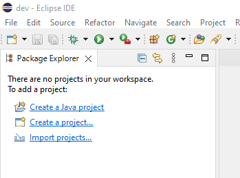
Inside the Package Explorer, click on Create a Java project.
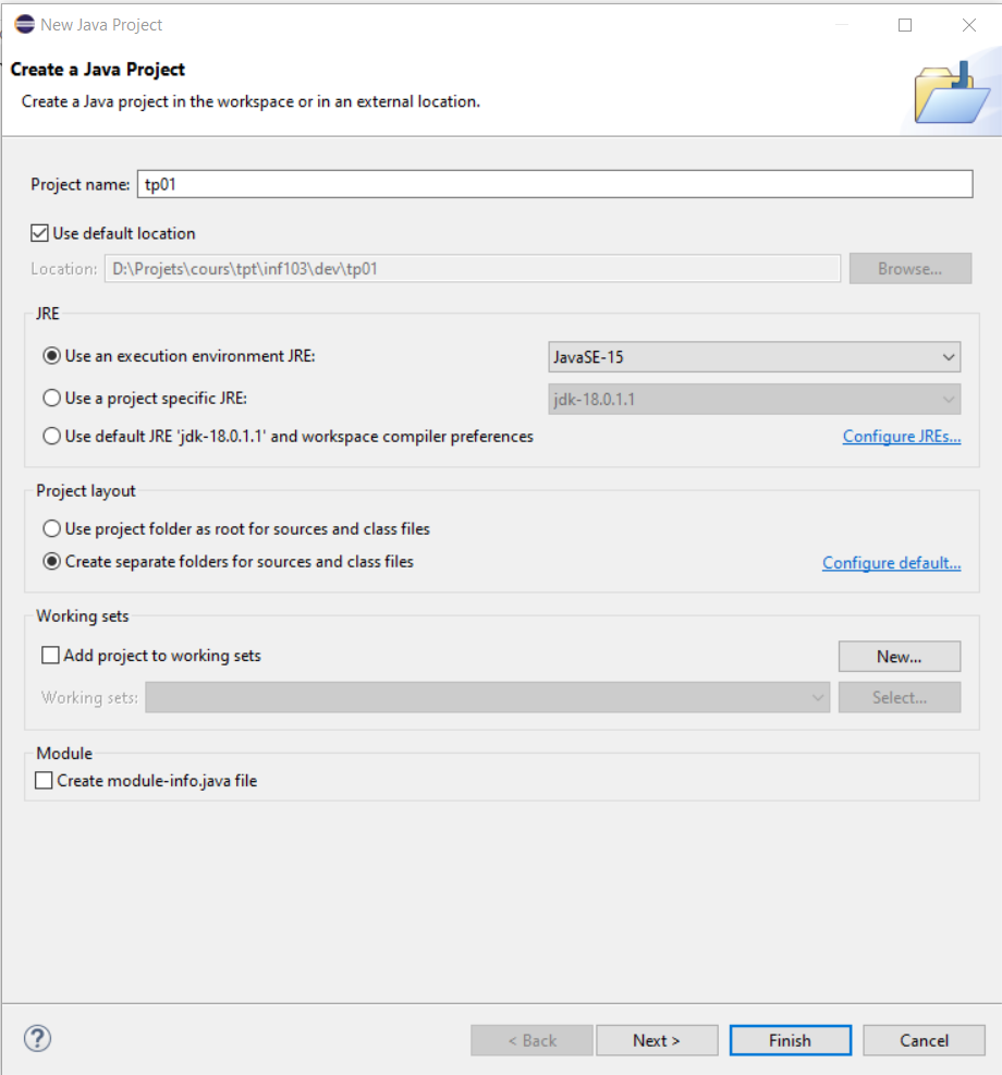
A new window appears (see below) asking you to enter the project name.
In the Project name field, enter tp01.
At the bottom of the window, locate the Create module-info.java file option (see Note 1). Ensure that this option is unchecked. If it is checked, uncheck it.
Leave all other options in the window unchanged.
Click the Finish button.

Note 1: The concept of modules, which we will not use for this course, is designed to improve the modularity of Java applications, particularly those of very large size.

The created project (tp01) appears in the Package Explorer panel (see below).
Click on the small triangle (>) to the left of the project name tp01. The triangle turns downward (∨) and the project contents are revealed (see below).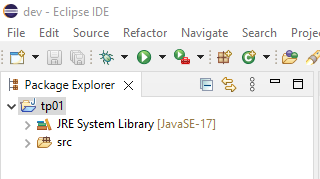
The src folder (abbreviation for source) appears, intended to contain the Java source code of your programs, along with the JRE System Library folder, which contains all the libraries that Java makes available to you. By clicking on the triangle (>) to the left of the JRE System Library folder, you can see the list of these libraries (see below).
These libraries are sets of predefined classes made available by Java. We will study some of them during the course. By clicking again on the triangle (∨) to the left of the JRE System Library folder, you can close this folder.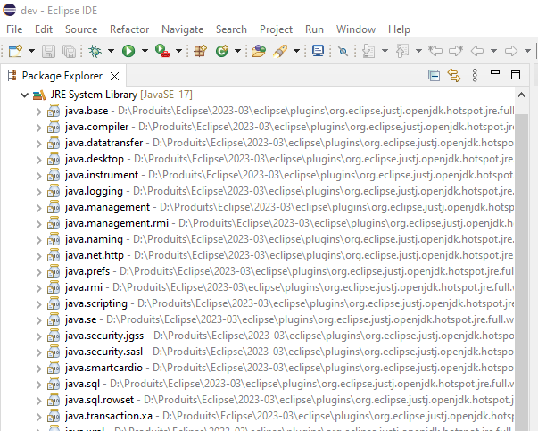

Creating a class

We are now going to create a class inside a package.

First, right-click on the src folder. In the menu that appears, hover the mouse over New. A submenu will appear; click on Package. In the window that appears, enter tp01 as the package name and click Finish.
Now, right-click on the newly created tp01 package. In the menu that appears, hover the mouse over New. A submenu will appear, hover the mouse over Class and click (see below).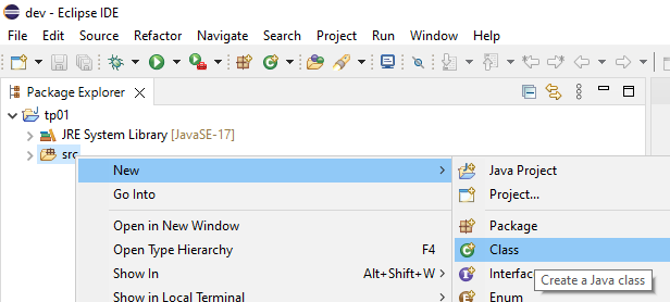
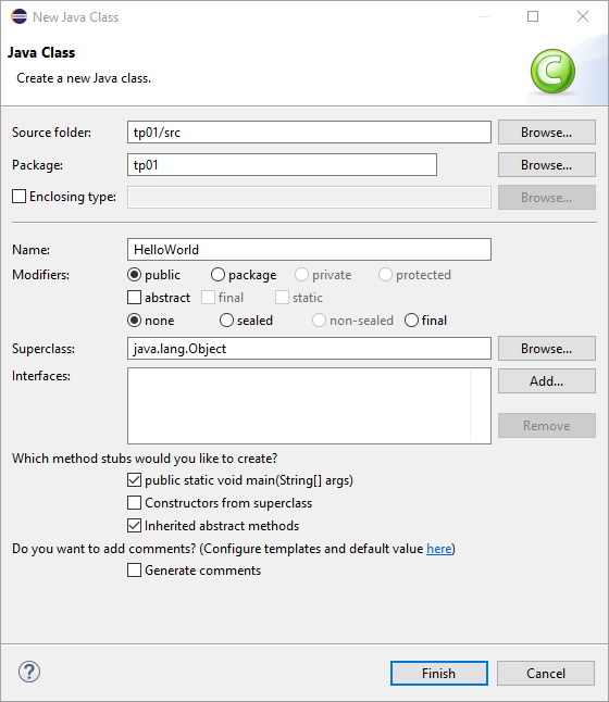
A new window like the one in the screenshot below appears.
In the Name field, write HelloWorld, then select the checkbox shown in front of public static void main(String[] args).
Click on the Finish button.

In the Package Explorer view, the class file named HelloWorld.java appears. In the central panel to the right of the Package Explorer, the Java code for this class is displayed. This panel also serves to edit the class code.

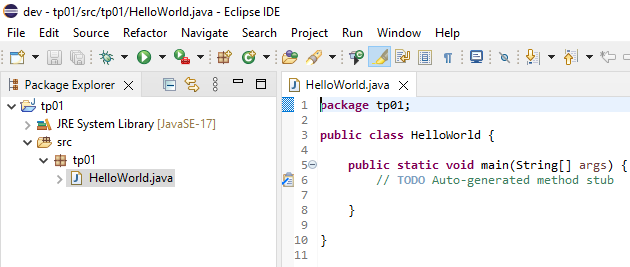
In this class, everything between the character strings /** and */ and everything between the character string // and the end of the line are areas dedicated to writing comments. These areas were generated by Eclipse. Also note the public keywords before the class and main method declarations. We will see the meaning of these keywords in a later lesson.

Remember: A method such as the main method is the one that will be executed when the program is launched.

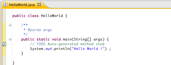
This method, generated by Eclipse, is empty. In its body, write the following instruction:
```
System.out.println("Hello World!");
```
You should get:
Save the file.

By default, Eclipse will compile the class as soon as its file is saved. The function of this instruction is to write the string "Hello World!" to what is called the Console.

To execute this program, click on the round green button with a white triangle inside located in the menu bar (shown below).

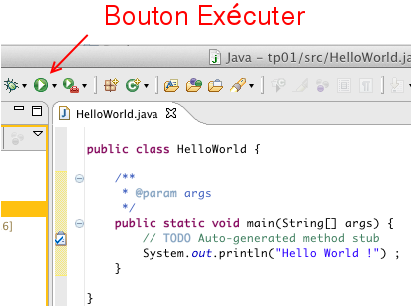
Eclipse will then execute the class, which will result in running the main method of your class, which serves as the entry point of the program. The Console panel will appear at the bottom of the code window. There, you will see the result of the print instruction. The program execution is immediately completed (shown below).

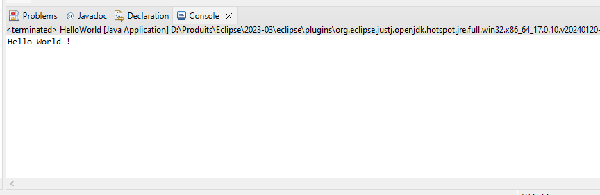
You have just executed your first program!

Compiling and executing a Java program via command line (without IDE)

As you have seen, creating a simple class and running its program is very easy with an IDE, which allows for more productive application development. But how would we do it without an IDE?

Java code is first compiled into binary code. The execution of a Java program is then done by interpreting this binary code using a JVM (Java Virtual Machine). The installation of this machine is carried out by deploying a JRE (Java Runtime Environment), which provides the virtual machine to run Java programs, or a JDK (Java Development Kit), which additionally includes the compiler (javac) and other utilities such as javadoc for automatic generation of documentation in the form of HTML pages.

These various executables are used via the terminal, a tool you have likely used before.

Compile your `Hello World!` program via the command line

As mentioned above, to compile and execute a Java program, you need a JDK environment specific to the given operating system (Windows, Linux, Mac). The virtual machine provided by this environment will interpret the compiled binary code to translate it into system-specific instructions. There are various providers of JDK/JRE environments, the most well-known being Oracle and the OpenJDK project.

The executables used to compile and execute Java programs are stored in a subdirectory named Java/<version_name>/bin, which is created in the operating system's program directory during the installation of the virtual machine.

To find out which version of Java is installed, type the following command in a terminal:
```
java -version
```
This version corresponds to the most recent version of the Java language supported by the virtual machine. For this exercise, please ensure that the Java version is higher than 1.8.

For a given version of Java, there are two types of virtual machine installations: the JRE installation mentioned earlier and the JDK (Java Development Kit) installation. The JDK installation includes everything contained in a JRE, as well as the Java source code and the javac executable used for compilation.

Installing the virtual machine

If you are working on your own computer (and not a school computer) and receive a message stating that the javac command is not found during the following exercise, install a JDK on your computer. You can use the JDK provided by Oracle or the one from the OpenJDK project.

Note 2: Recent versions of Eclipse include their own JDK, which can also be used. If applicable, it will be located in the Eclipse installation directory under:

../eclipse/plugins/org.eclipse.justj.openjdk.hotspot.jre.full.<version>

However, this may depend on how Eclipse was installed (for example, via an installer or an archive) or even on the operating system.

To find out the directory of the JVM used by Eclipse, simply click on the menu Window > Preferences. In the dialog box that appears, select the branch Java/Installed JREs, as illustrated in the screenshot below. The right side of the window will indicate the installation directory of the JVM used by Eclipse.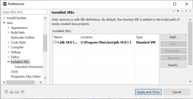
If you have not already done so, in a terminal, navigate to the src directory of your "Hello World!" program's Eclipse project.
To find this directory, in Eclipse, select the src folder in the package explorer, then right-click and select the Properties menu. In the window that appears, select the Resource branch. The src folder's directory is displayed on the right side of the window as indicated by the Location label (Shown bellow). A button also allows you to open a file browser directly positioned in the directory.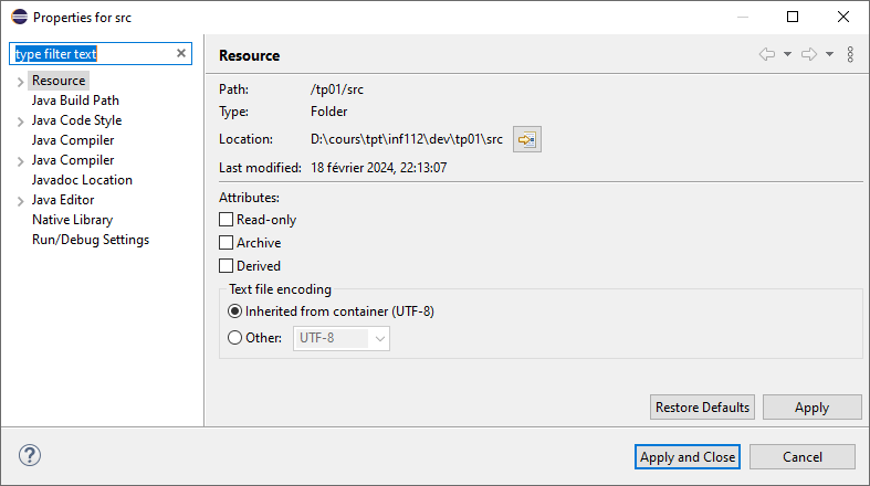
Then type the command
```
javac tp01/HelloWorld.java
```

Examine the contents of the src/tp01 directory containing the Java file. You will see that running the javac program has produced another file named HelloWorld.class from the HelloWorld.java file. This file contains the binary code generated by compiling the Java code.

It is possible to specify a directory (different from src) to javac for storing compiled files. For example, during compilation, Eclipse will store the compiled files in a different directory named bin (for binary) located at the same level as src in the project directory.

Execute your `"Hello World!"` program

The HelloWorld.class file containing the compiled code can now be executed by the virtual machine.

To do this, run the java executable with the class name as a parameter. While still being in the src directory, type the command:
```
java tp01/HelloWorld
```
You should see the following string displayed in the terminal.
```
Hello World!
```
It is also possible to perform these two operations ( that is, Nr. 6 and 7) in a single command with the Java executable. First, delete the compiled HelloWorld.class file and verify that it has been deleted. Then, type the command (see also Note 3):
```
java tp01/HelloWorld.java
```
You will see the string Hello World! displayed in the terminal.
```
Hello World!
```

Note 3: Executing the program in this way, note that the compiled file was not saved to disk. It was simply created and then executed without being saved. Thus, it is preferable to first compile a program using javac (which is what Eclipse does), as the program can then be executed as many times as desired without recompiling.

Note 4: These commands work for a class contained in a package¹ named tp01 (that is, its .java file is directly in the tp01 subdirectory of src). If you have declared your class in another package (for example, a package named test), its .java file will be contained in a subdirectory named test of src. To execute this class, you must position yourself in the src directory and prefix the class name with its package name test instead of tp01.

If you try to execute the class in the test subdirectory, you will see an error message such as

Error: Could not find or load main class HelloWorld

You must therefore verify that you are launching the commands from the src directory.

These simple commands show us how Eclipse (or any other IDE) compiles and executes a Java program for us. In Eclipse, compilation is executed each time a Java file is saved. Thus, when a project contains multiple Java files, Eclipse will only recompile the modified files and those that depend on them, which is called incremental compilation, minimizing the compilation time.

We will cover the concept of packages in a later course.

Committing your project to GitLab (Optional)

Note: This step is optional for this lab but highly recommended, as you will need to use Git throughout the course and for your final project.

Now that you have created your first Java project, it is important to learn how to version your code using Git and store it in a remote repository on GitLab. This will allow you to track changes, collaborate with others, and back up your work.

Creating a GitLab repository

Go to GitLab and log in with your school credentials.
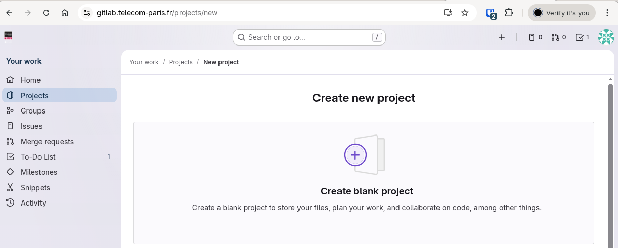
Click on New project (or the + button in the top menu).

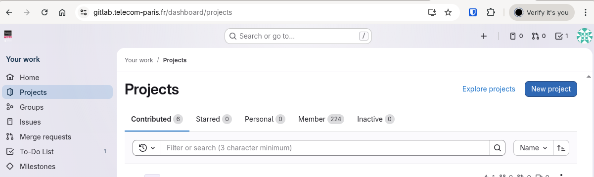
Select Create blank project.

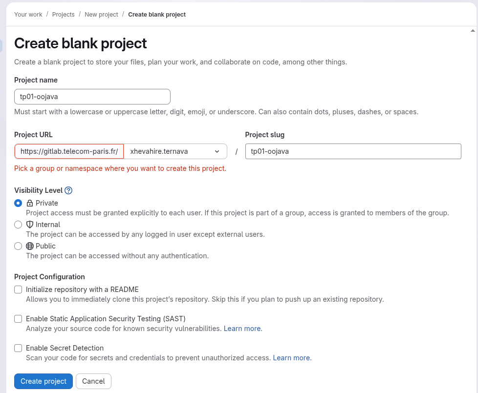
In the Project name field, enter your project name following the format: tp01-oojava.
Set the visibility level to Private.
Uncheck Initialize repository with a README (we will initialize it locally).
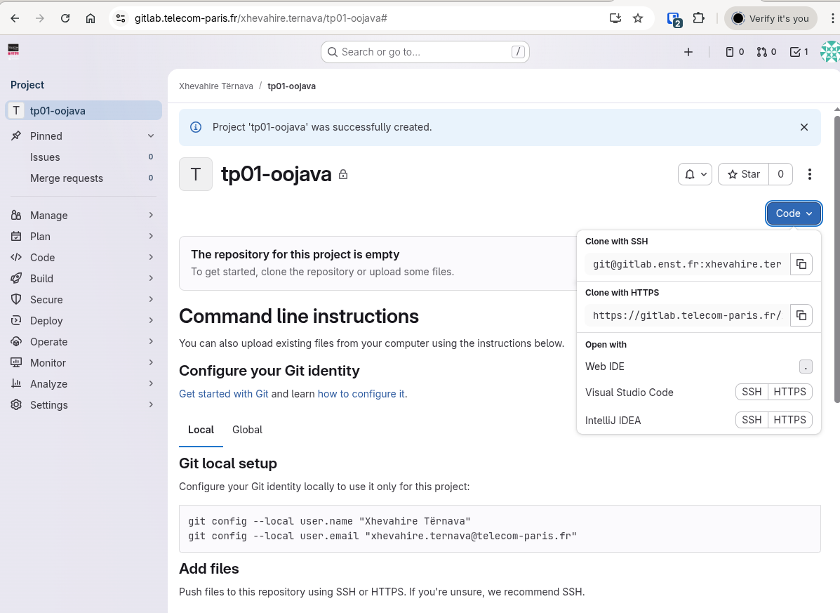
Click Create project.

GitLab will display a page with instructions. Keep this page open as you will need the repository URL.

Initializing Git in your project

Open a terminal and navigate to your Eclipse project directory (the parent of the src folder).
Initialize a Git repository:
```
git init
```

Configure your Git identity (if not already done):

git config user.name "Your Name"
git config user.email "your.email@telecom-paris.fr"

Create a .gitignore file to exclude compiled files:

echo "bin/" > .gitignore
echo "*.class" >> .gitignore

Committing and pushing your code

Add all files to the staging area:
```
git add .
```

Create your first commit:

git commit -m "Initial commit: Hello World program"

Add the remote GitLab repository (replace <your-repository-url> with the URL from step 8):
```
git remote add origin <your-repository-url>
```
Push your code to GitLab:
```
git push -u origin main
```
Note: If your default branch is named master instead of main, use:
```
git push -u origin master
```
Refresh your GitLab project page in the browser. You should now see your project files in the repository.

You have successfully versioned and pushed your first Java project to GitLab!

TP 2: Programming a `Robot` class

Overview

In this assignment, we will learn to code a first class used to model a robot, which will ultimately serve to model the production factory in the simulator you must produce as part of this course’s project.

Because programming software is more familiar with English than other languages, it can be complicated to work with class, method, or attribute names written in French. This is why you will always use English words in your code.

The internet is a reference for Java programming. You will find programming examples for everything you want. Just use a search engine with the right keywords. You will also find tutorials on using Eclipse, the vast majority of which are in English. If your version of Eclipse is in French, it may require some effort to find your way around.

In this lab, you will learn to:

Getting started with the `robotsim` project

Launch Eclipse from your operating system's menus.
Using the File > New > Java Project menu, create a project named robotsim.

Note 1: The sources for this project should be archived in a Git repository that will be provided to you and will constitute your development project to be submitted at the end of the course.

Creating a `Robot` class

In the src folder of the robotsim project, as done for the HelloWorld class in the previous assignment, create a class named Robot. This class will be used to model the concept of a robot within a washer production factory, similar to the one you will develop for the course project.
Among the attributes of the Robot class, we must have:
- An attribute named name of type String.
- An attribute named speed of type double.
Use the Java code editor to declare these attributes in the Robot class.
We will now write a constructor for this class. This constructor should initialize all fields. You can code this constructor directly in the class editor or use the IDE:

(a) Right-click in the editing window of the Robot class or on the Robot.java file in the Package Explorer.

(b) A menu appears; move the mouse over Source.

(c) A second menu appears; click on Generate Constructor using Fields (do not select Generate Constructor from Superclass; this concept has not yet been covered in the course).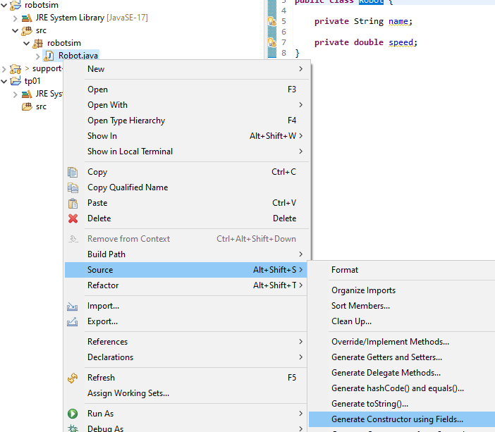
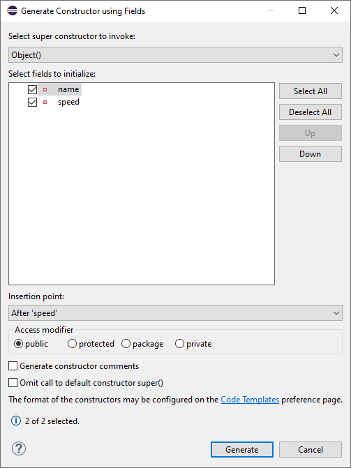
A window appears that allows you to customize the constructor:
Verify that both attributes are selected. The Insertion point of the constructor in the class can be left as is or selected to be, for example, after the declaration of the attributes.
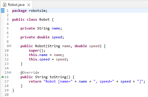
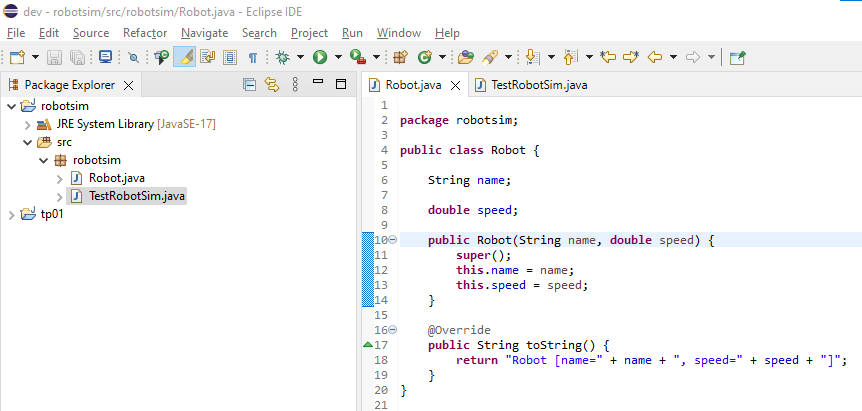
Click on the Generate button. You then get a modified class: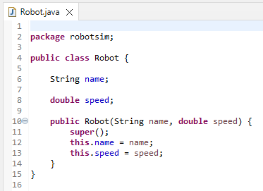
Before leaving a class to edit another, always save the class currently being edited. The Save button is located in the menu bar of Eclipse.

Creating a `TestRobotSim` class

Now, let's generate a second class called TestRobotSim containing a main method, like in the HelloWorld class from the first lab (TP01).
In this main method, create an object of type Robot with the instruction:
```
Robot myRobot = new Robot("Robot 1", 5);
```
Then print the object in the console with the instruction:
```
System.out.println(myRobot);
```
Then run the program. What do you notice about the output of the class?

Customizing object display with `toString`

We can see that Java does not know how to display an object of the class. It knows how to display strings, numbers, etc., but it does not know the class, which is our invention. When Java does not know how to display an object, it displays the name of the object's class, here Robot, followed by the $@$ symbol (at sign), followed by the memory address of the object expressed in hexadecimal (base 16).

If we want Java to be able to display an object of the class correctly, we need to provide a toString() method returning a string representation to display / print the object. This method has the following header:

public String toString();

To generate this method in the Robot class, you can use the IDE:

Right-click on the editing window of the Robot class.
A menu appears. Move the mouse over Source.
A second menu appears; click on Generate toString(). A window appears to offer you the generation of a toString() method: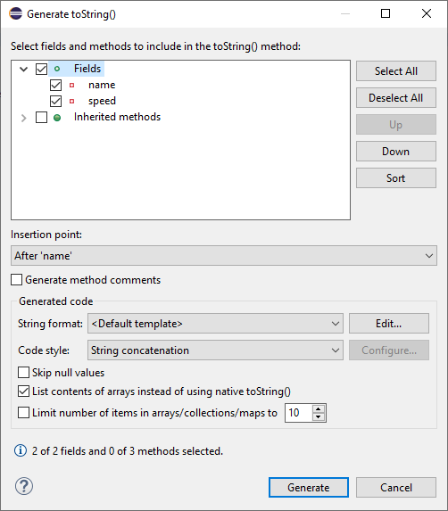
The method that will be generated will calculate a string that includes the name of the class followed by the value of the attributes. In this window, it is possible to add other properties to the display. Click on the Generate button.
The class is modified:

The @Override annotation, placed just before the method, indicates that this method is overriding an inherited method. We will cover this in the course later.
Run the program again. Is the object's display more understandable and useful now? You should get this in the Console view: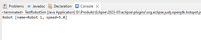

Redefining the display of robots

Now let's improve the default toString() output with a more human-readable format.

Execute your program from the previous lab (TP01) to verify that everything still works well.
Modify the toString() method of the Robot class so that it returns the string formed as follows:
```
My name is Robot 1 and I move at 5.0 km/h.
```
Run your program and verify that everything works correctly.

Utility of an IDE

In this lab, you wrote little code manually. This will not always be the case. The development environment allows us to perform standard coding tasks (generation of constructors, getters, setters, toString(), etc.) with just a few mouse clicks.

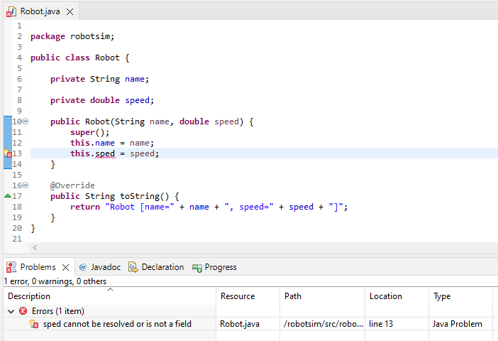
The IDE also notifies you of compilation errors and warnings via the Problems view shown in the following screenshot. In this view, double-clicking on an error in the list will take you directly to the position of the error in the Java code editor.

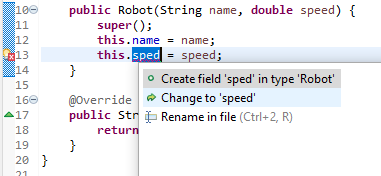
Moreover, in the margin of the code editor, error correction suggestions can be proposed by the IDE by clicking on the light bulb, as illustrated by the screenshot of the following window. In this example, the speed attribute name was incorrect.

It is also possible to automatically rename code elements such as class or variable names (refactoring).

All these features are very useful in an industrial development environment as they greatly improve the programmer’s productivity. You should not hesitate to use them, although you should always understand the generated code. Indeed, the IDE will not program algorithms for you, although extensions such as Copilot (a paid tool) using artificial intelligence could potentially be useful.

TP 3: Modelling a factory containing robots

Overview

For this lab, you will continue working in the same project as the previous lab, TP02 (named robotsim), which will eventually contain all the sources for your development project in this course.

Remember: This project will be submitted at the end of the course.

In this lab, you will learn to:

To model a goods production factory, you will add a new class named Factory.

But first, launch Eclipse to work on the same robotsim project.

Encapsulating the `Robot` class data

We have seen in class the importance of encapsulating data. This is done using the private visibility keyword in Java. Modify the visibility of the attributes in your Robot class, then generate accessors for these attributes, considering that a robot's name cannot change during its existence, which is not the case for its speed. Just like for the generation of the toString() method in the previous lab, the IDE can automatically generate these accessors for you.

Creating a `Factory` class

By right-clicking on the robotsim package and then selecting the New > Class menu, create a class named Factory.
Since a factory has a name and must contain multiple robots, declare in this class a name attribute as for your Robot class and an attribute named robots of type ArrayList<Robot> to contain the factory's robots. Don't forget to encapsulate these attributes using the private qualifier. You should get this: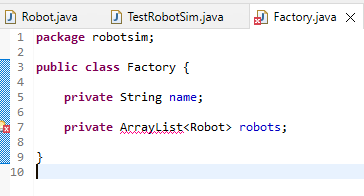

Import declaration

A red mark indicating an error has appeared in the left margin of the code editor. When hovering over this marker with the mouse, the error is displayed:

Indeed, the ArrayList class is not known by default. As seen in class, you must import this class using the declaration:
```
import java.util.ArrayList;
```
This declaration must be placed at the beginning of the class file. Here again, the IDE can help you. By clicking on the red error mark, the IDE will offer you different possible solutions:

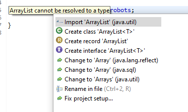
The first solution is of course the correct one. Move the mouse and click on Import 'ArrayList' (java.util). The import declaration is then automatically added to the class.

Writing the constructor

As we have seen in class, by default the robots attribute is initialized with the value null. We need to specify a constructor to initialize the attributes of a class with suitable values. Consult the Javadoc of the ArrayList class to know the constructors of this class. The constructor must create and assign the ArrayList for robots, and take the name as an argument.

Write a constructor for your Factory class.

Hint: Your constructor should look like this:
public Factory(String name) {
    this.name = name;
    this.robots = new ArrayList<Robot>();
}

Adding a robot to the factory

Write a method in the Factory class that will allow adding robots to the factory. It will have the following signature:
```
public boolean addRobot(String name)
```
This method should first verify that the name of the new robot named name is unique among the names of robots that have already been added to the production factory. If the name is unique, then the method should create a new Robot object with the given name and a speed of 0.0, add it to the factory's list of robots, and return the boolean value true. Otherwise, the robot will not be added to the factory and the boolean value false will be returned.

Verifying the uniqueness of robot names

Write a method in the Factory class that will verify the uniqueness of a robot name passed as a parameter. This method, which will be called by the addRobot() method, will have the signature:
```
private boolean checkRobotName(String name)
```
It should iterate through the list of robots to verify that none of them has the same name as the one passed as a parameter. The method should return true if the name is unique (i.e., no existing robot has it), and false otherwise.

Displaying the factory and its robots to the console

Write a method in the Factory class with the following signature:
```
public void printToConsole()
```
This method will display the name of the factory as well as the list of its robots to the Console.

Testing the methods

In the main() method of the TestRobotSim class created in the previous lab, add instructions that will:
- Create an object of the Factory class.
- Add a few robots to this object. Make different trials with some robots with identical names to verify that your program works correctly.
- Display the Factory class object to the Console.
Execute your program with different sets of robots and verify that what is displayed on the Console is correct.

Organizing classes into packages

You have probably noticed when you created the Robot and Factory classes with Eclipse that it put them in a package named robotsim, which has the same name as the project.

This organization of classes is not ideal because, as seen in class, it is preferable to group classes that perform a common functionality of the application within the same package.

The Factory and Robot classes perform the function of modelling the production factory. They will therefore be grouped within a package named fr.tp.inf112.robotsim.model. What about the TestRobotSim class?

To change the package of a class, it is not enough to rename the package declaration in the class. Indeed, Java requires that the class file be located in a directory tree of the file system equivalent to the class package name, after converting the "." characters of the package name to "/" characters.

Again, the IDE can automatically change the package declaration of the class and move its file to the correct corresponding subdirectory.

To do this, select the class(es) in the package explorer and right-click. In the menu that appears, select Refactor > Move...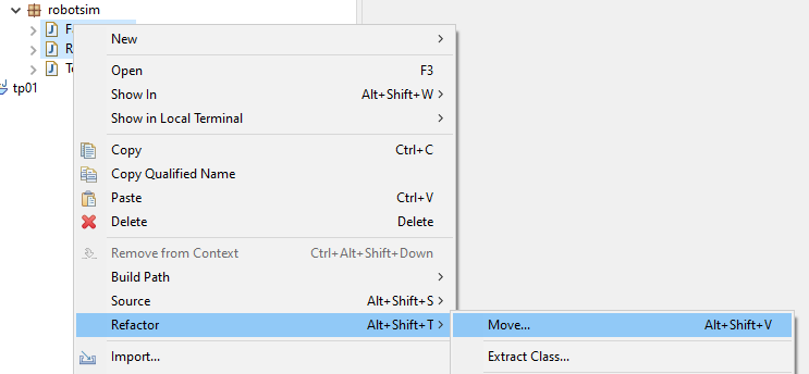
In the dialogue box that appears, enter the desired package name and click Finish.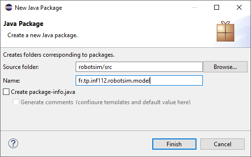

Do not forget to also change the package of the TestRobotSim class. Since it is not part of the model, move it to a separate package, for example fr.tp.inf112.robotsim.app.
Run the TestRobotSim class again to verify that your program still works correctly after reorganizing your classes.

TD 1: Design exercise - Model the structure of a robotic factory

Overview

In this design exercise, you will work in teams to create a class diagram modelling the structure of a robotic production factory. This exercise introduces the project you will develop throughout this course.

In this exercise, you will learn to:

Project: Develop a simulator for a robotic production factory

Inspired by the Cyber-Physical Systems Laboratory of the Hasso Plattner Institute (Potsdam, Germany)

https://www.hpi.uni-potsdam.de/giese/public/cpslab/

Why this system?

Allows the implementation of essential OO concepts.
- Delegation/non-intrusion, inheritance, polymorphism, abstract classes, ...
Allows the implementation of interfaces for integrating different software components.
- A graphical interface will be provided, and integrating this component will allow visualizing the simulation, making development more fun.
Illustrates several design patterns and the importance of software architecture.
Can be extended to implement advanced aspects (2nd year courses):
- Data persistence
- Parallel programming and resource access synchronization
- Distributed applications
- and more...

Project requirements

R1: Model a simplified robotic production factory containing these elements:
- Factory, robots, robot charging stations, rooms and doors, work areas, production machines, and conveyor.
R2: Simulate the behaviour of robots transporting produced goods (washers) from one place to another within the factory:
- For each robot, provide a list of positions to visit in the factory, and the robot must move to visit them in succession.
- Robots must avoid obstacles on their path.
R3: The factory and its simulation must be visualized through a graphical user interface.
R4: The model (data) must be saveable to disk.
R5: The application must handle exceptions that may occur during the execution of the program:
- For example, when there are issues accessing data on disk.

Optional, if you have enough time:

R6-opt: Simulate the robot's energy consumption. If a robot reaches a specified minimum energy level, it must move to a charging station and stay there for a certain time to recharge. (Assumption: Energy consumption is proportional to the robot's speed).
R7-opt: Doors will open and close automatically when a robot needs to enter a room.

Development requirements

R8-dev: Implement good programming practices discussed in class:
- Definition and organization of classes.
- Naming conventions.
- Comments and code formatting.
R9-dev: The architecture must follow the MVC (Model-View-Controller) pattern as presented in class.

What is not required

The details of the features to be implemented for the project will be provided in each of the lab instruction documents.
Given the limited time available, several aspects of the simulator will obviously not be considered for this project; they will be covered in an advanced Java programming course in the second year.
- For example:
  - Parallelism and concurrent access to resources (synchronization).
  - Distributed application.
  - Database.
  - Etc.
This system is only intended to illustrate the concepts and good programming practices taught in the CSC_3TC36_TP course. It is not meant to be a professional simulator.

Example of robotic production factory structure

https://www.hpi.uni-potsdam.de/giese/public/cpslab/detailed-laboratory-description/

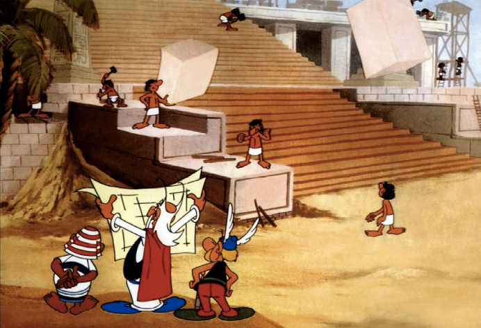
Importance of design: Another example of a very (very) simple system

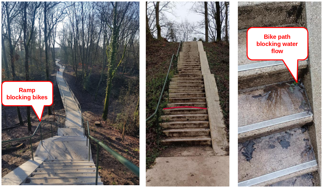
Bridge of the Troche quarry:
- On the path to catch the RER B at the Guichet station from the school.
Find two design errors.

Answer

Importance of design

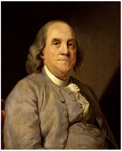
"If you fail to plan, you are planning to fail!" -- (Benjamin Franklin painted by Joseph-Siffrein Duplessis)

Guided design exercise

In groups of 2 or 3 students, draw a class diagram to model the structure of the robotic factory:

Draw on paper or use another tool of your choice.
20–30 minutes of teamwork.
Presentations from some teams on the board.
Discussions and iterative improvements of the class diagram.
Note: Focus only on the structure of the factory; the behaviour (modelled by class methods) will be specified in a future lab session.

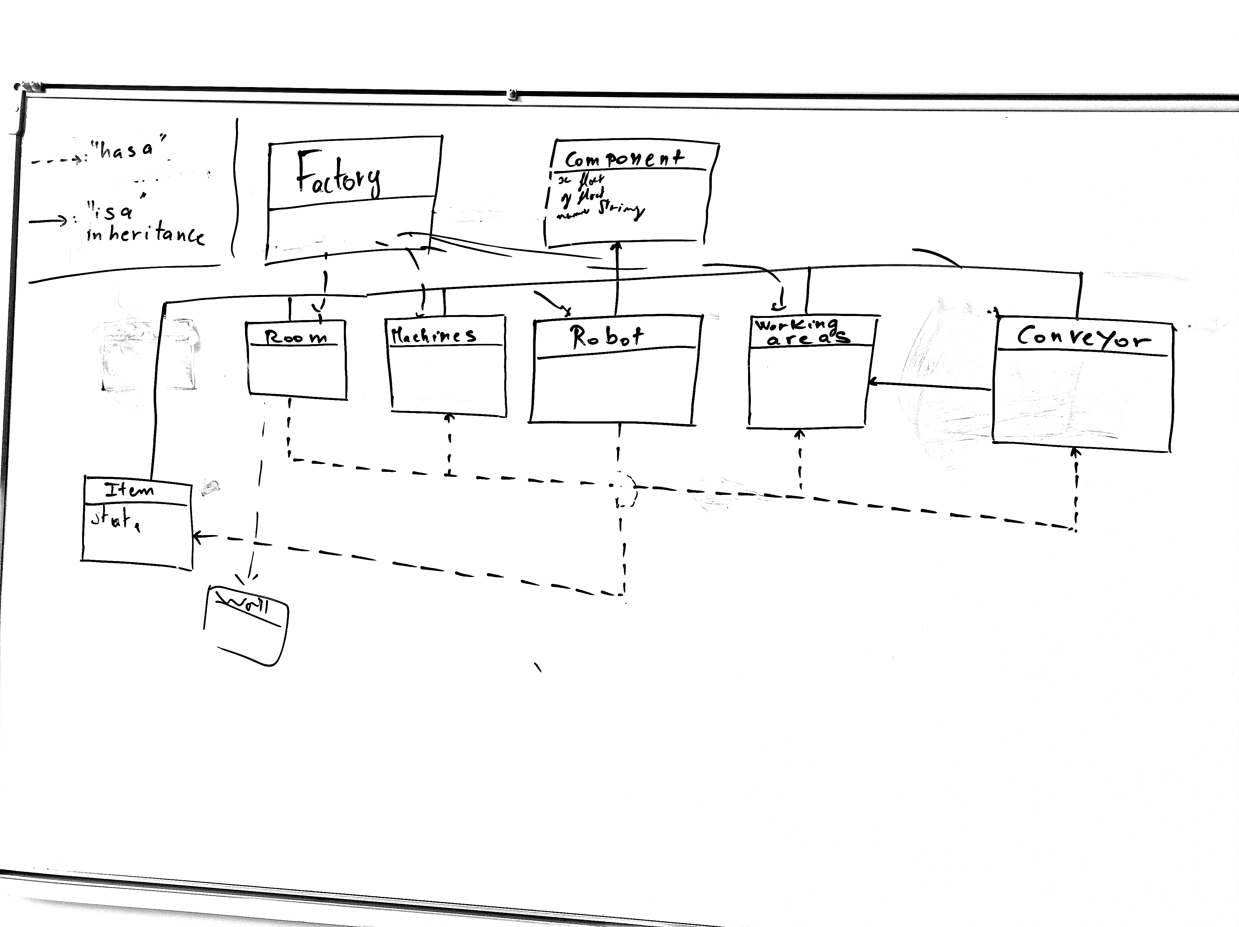
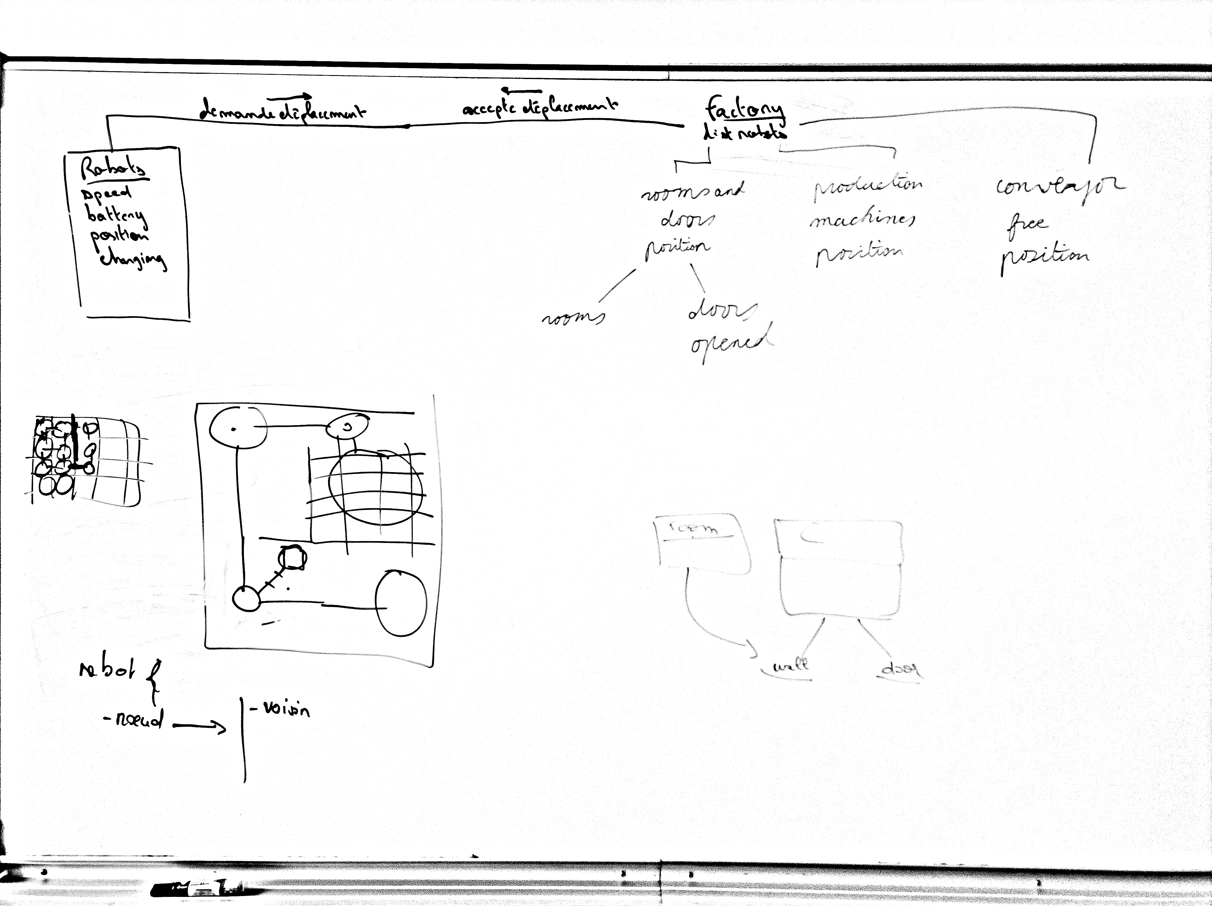
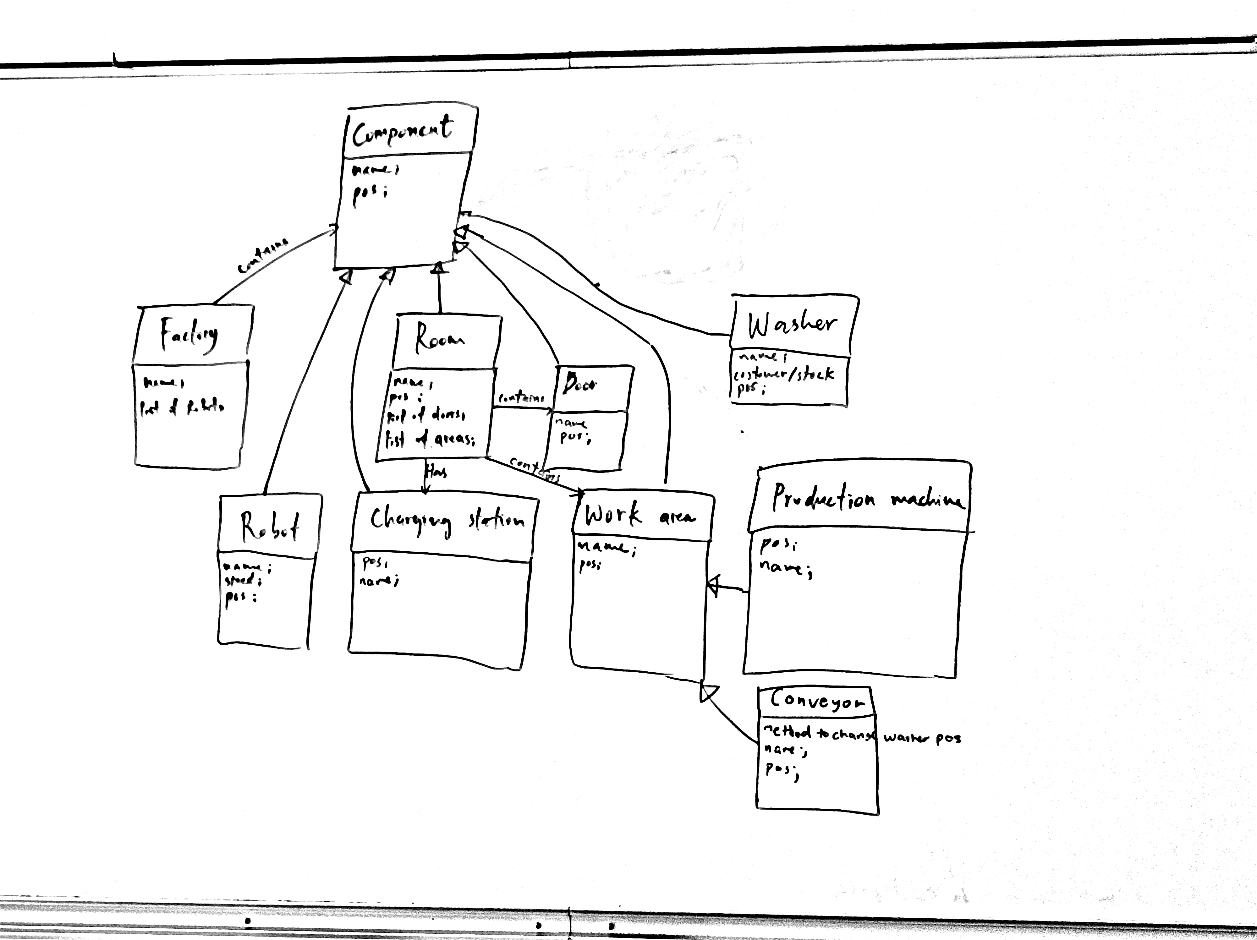
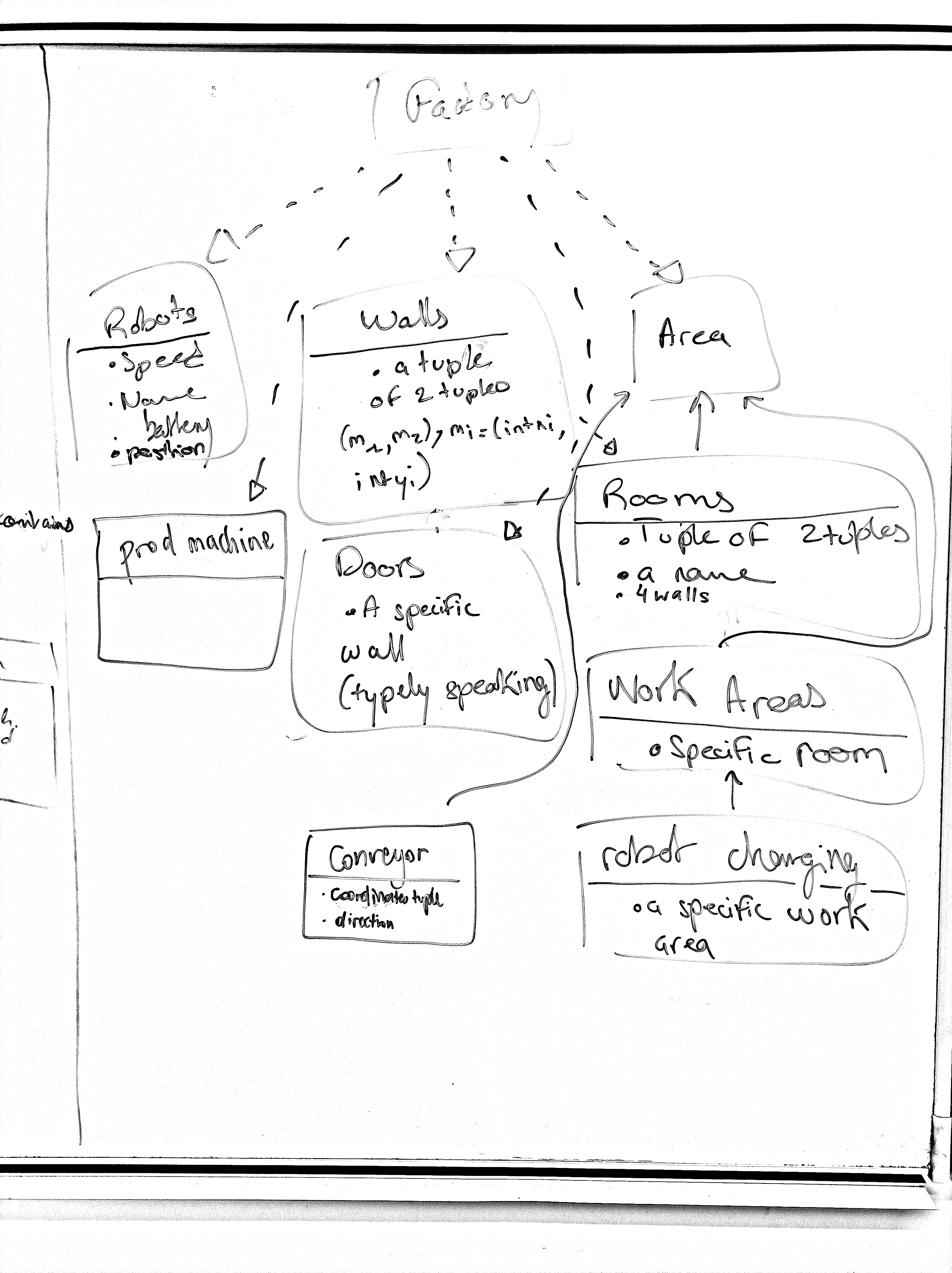
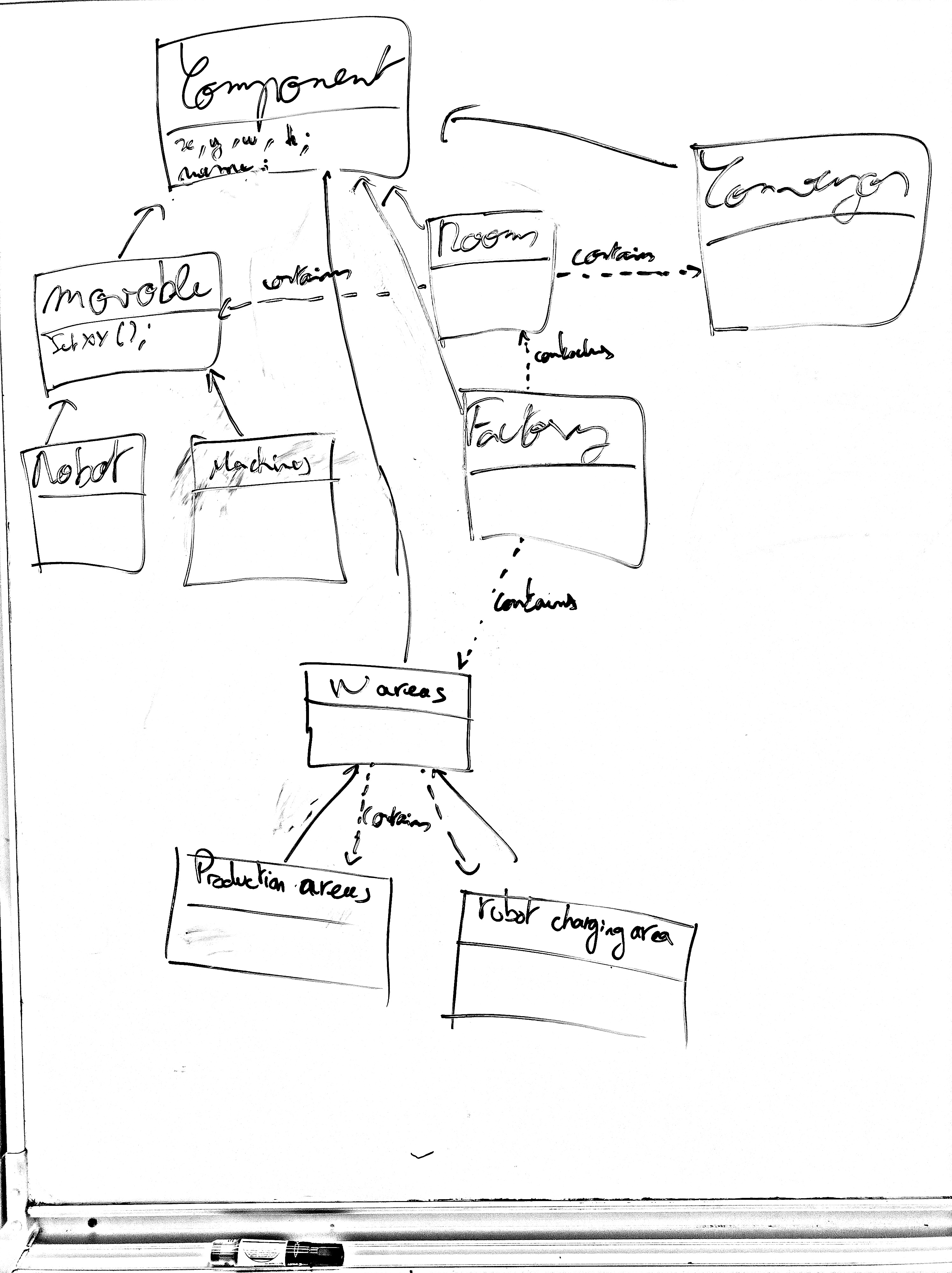
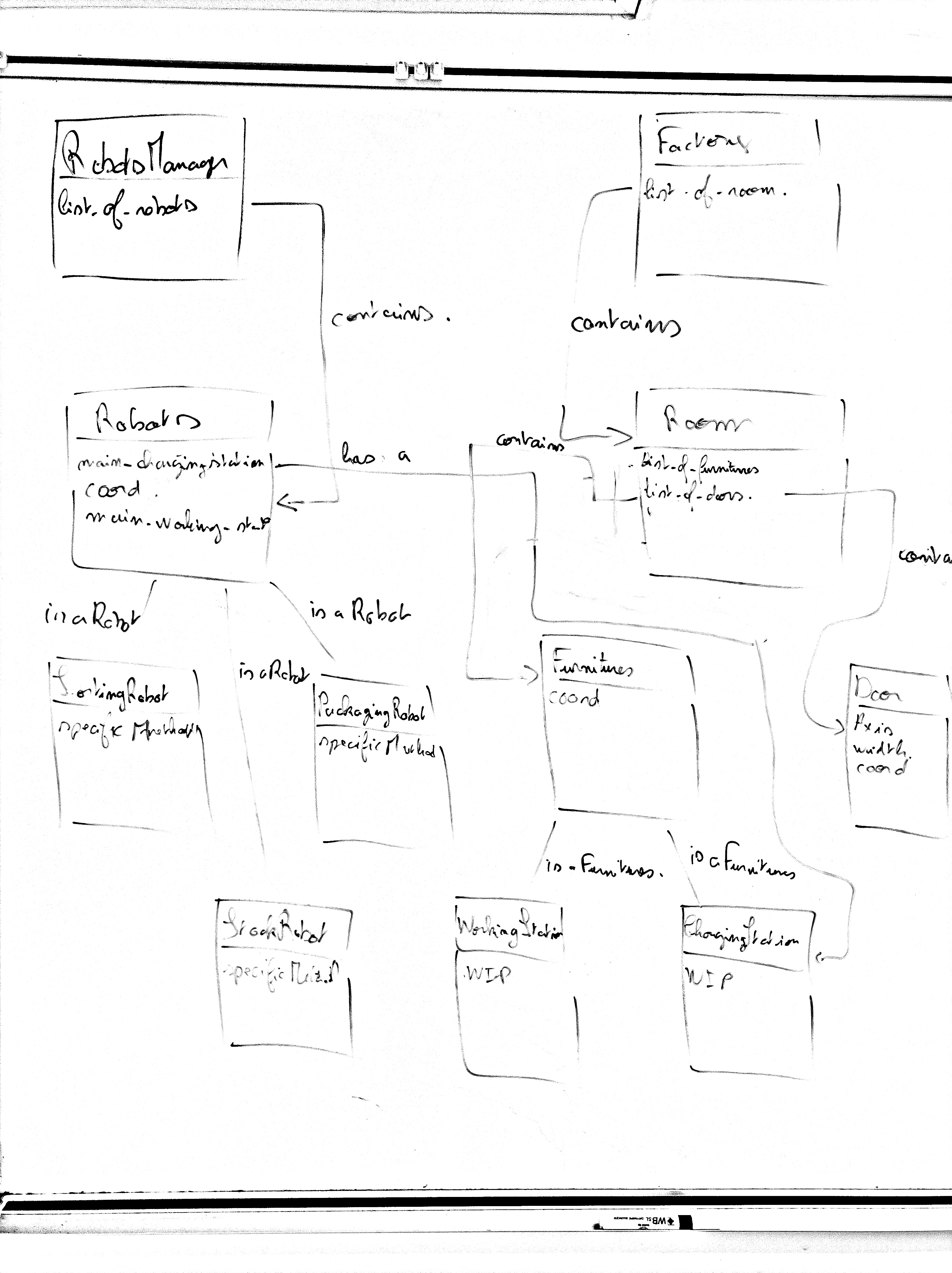
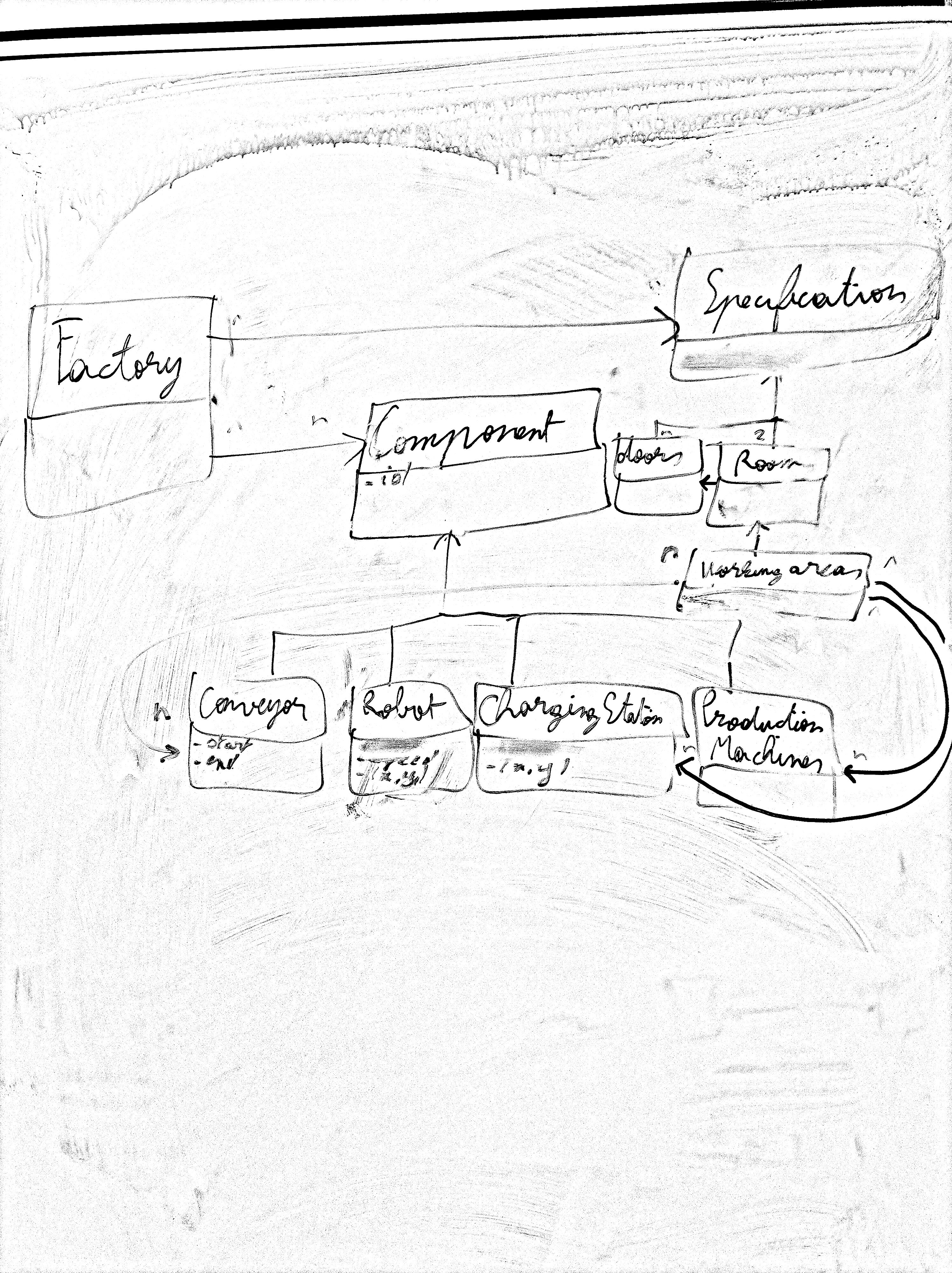
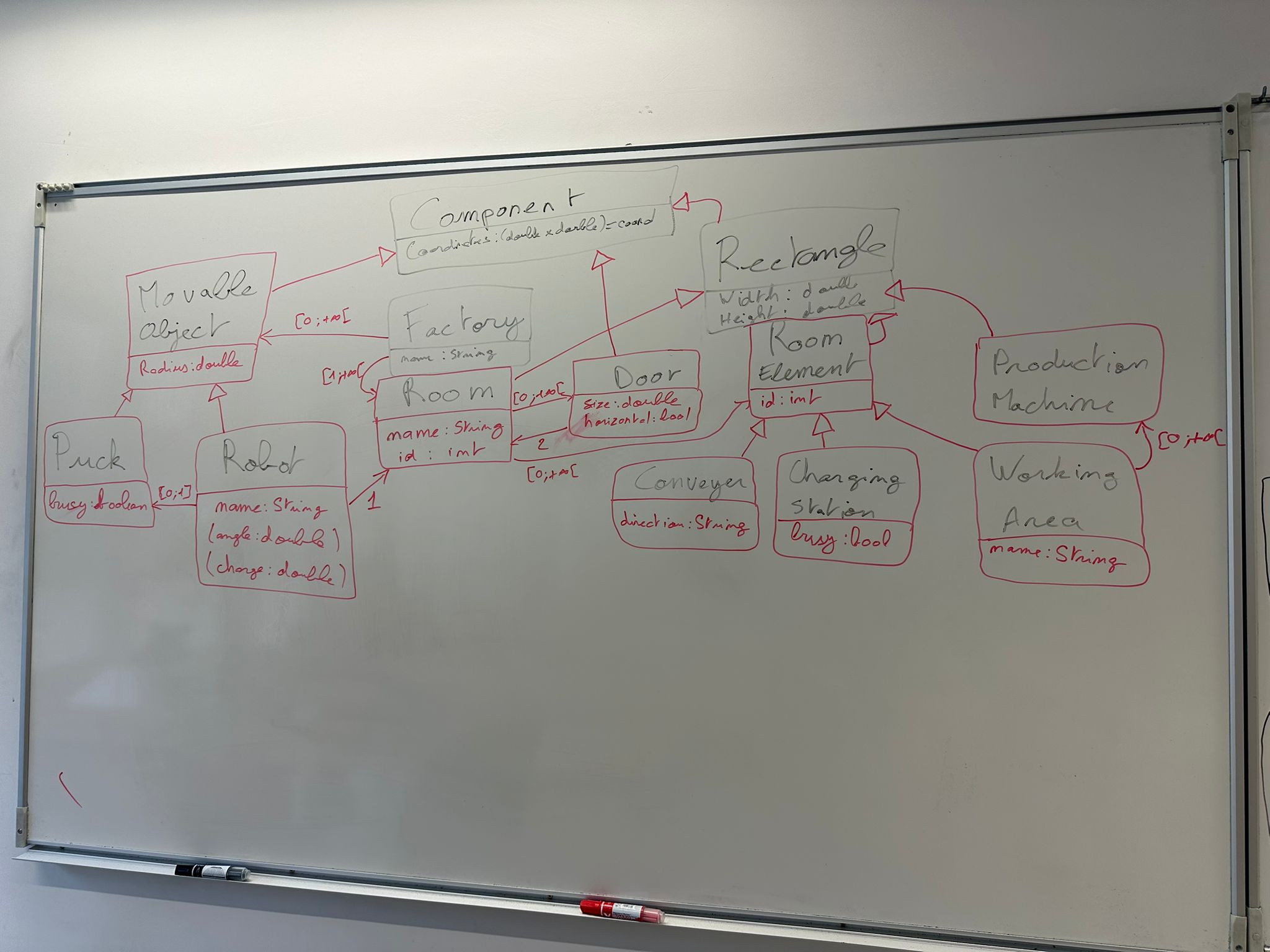
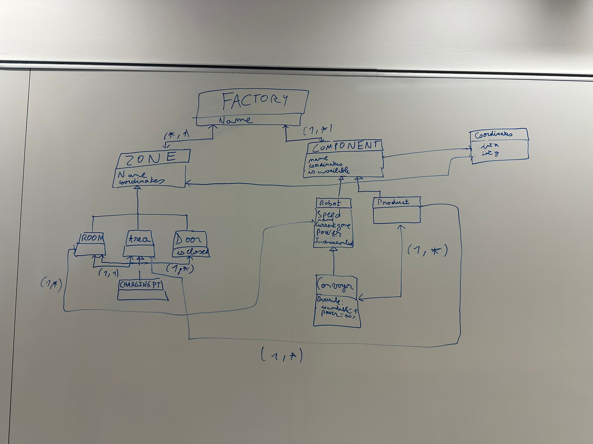
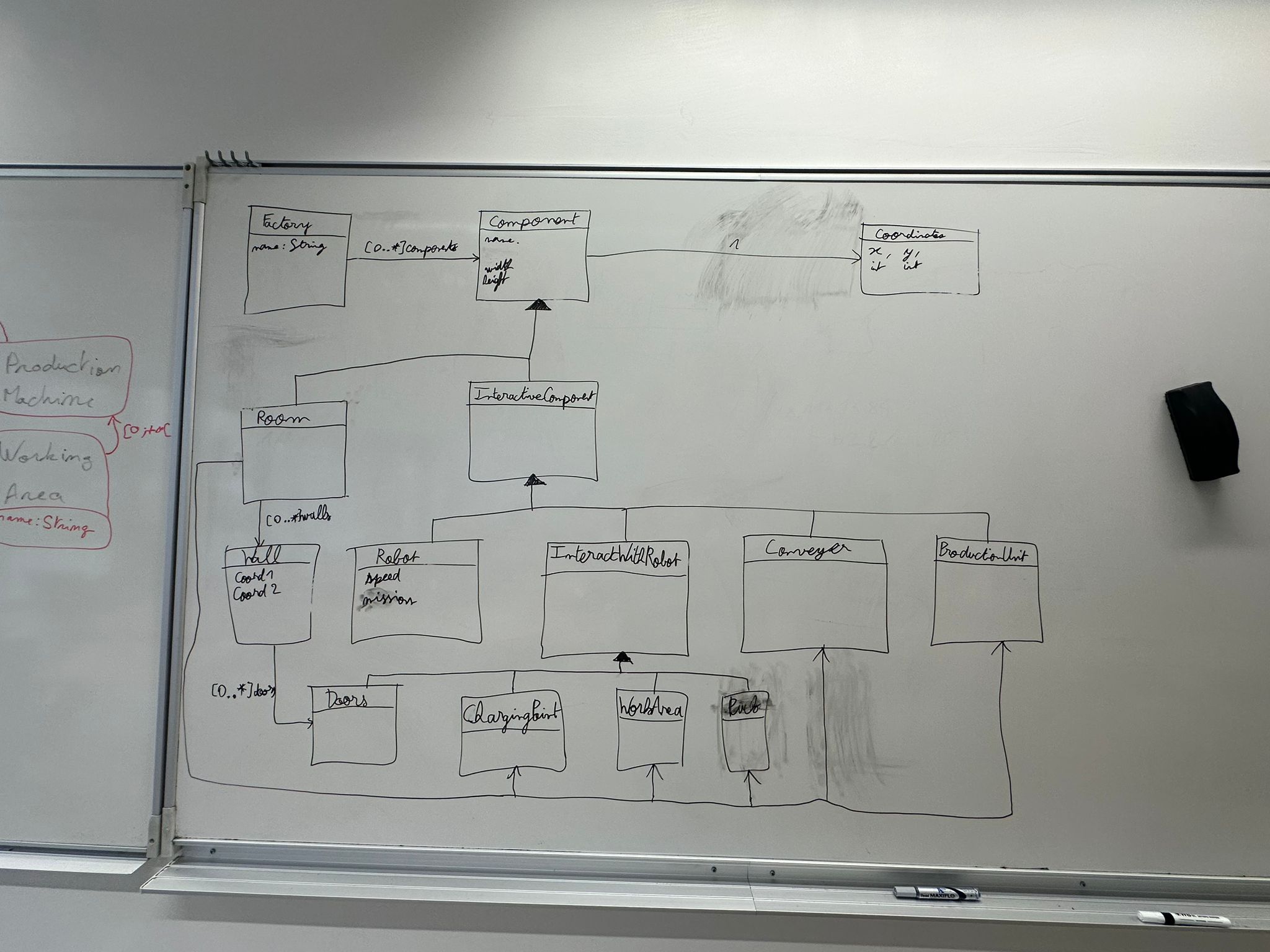
Student Class Diagrams — TD1 (2026)

UML class diagrams designed by student teams during the guided design exercise.

Tip: Click on any image to view it in full size.

Team EN-1

Team EN-2

Team EN-3

Team EN-4

Team EN-5

Team EN-6

Team EN-7

Team EN-8

Team FR-1

Team FR-2

Team FR-3

TP 4: Coding the robotic factory model in Java: Structural view

Overview

The goal of this exercise is to code in Java the class diagram you drew during the previous practical session (TD). Photos of the various class diagrams produced by the different teams have been uploaded to the course's Moodle website. You are free to use these as inspiration for building your own model of the factory, keeping in mind that these diagrams are not perfect, and there is no single way to model a system.

Moreover, these diagrams were created before you had learned all the concepts and best practices in modelling introduced later in class, such as abstract classes and the Single Responsibility Principle. Translating the class diagram into Java thus provides an opportunity to improve your design using these concepts and best practices, and to enhance it where necessary.

In this lab, you will learn to:

Robotic factory

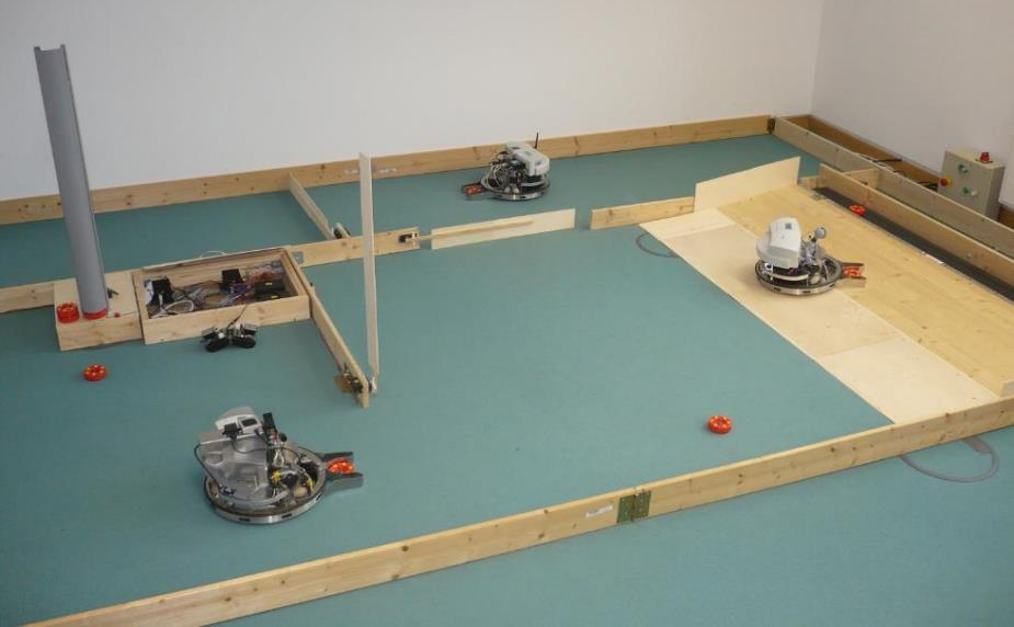
As discussed in class, the robotic factory is inspired by Hasso-Plattner Institute’s Cyber-Physical Systems Lab (Figure 1).

Figure 1. The robotic factory from the Hasso-Plattner Institute’s Cyber-Physical Systems Lab.

Figure 1. The robotic factory from the Hasso-Plattner Institute’s Cyber-Physical Systems Lab.

Factory overview

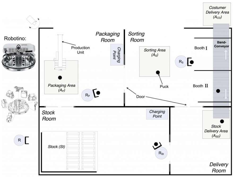
As illustrated in the floor plan in Figure 2, the factory consists of various rooms where machines are installed. These machines are designed to perform specific processing tasks on the washers produced by the factory.

Inside this factory, robots transport washers between the different production machines. When needed, these robots can go to charging stations to recharge their batteries until they have enough energy to resume their work.

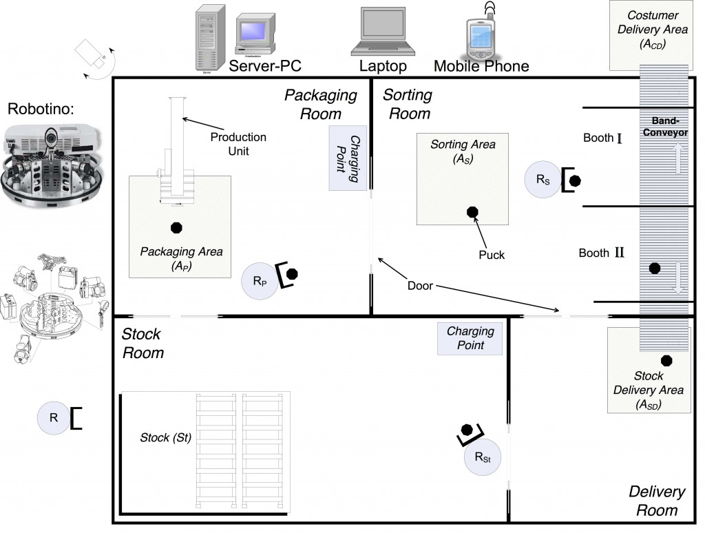
Figure 2. Floor plan of the robotic factory

Figure 2. Floor plan of the robotic factory

System simulation

When designing systems such as an automated production factory, simulation is very useful for evaluating various properties such as:

The amount of goods that can be produced per unit of time.
The number of robots required to transport goods from one machine to another.
The battery capacity required for the robots to produce this quantity of goods without spending too much time at the charging stations.

The simulator you will develop for this project will visualize the behaviour of the robotic factory. Specifically, this includes displaying events like robots moving through the building while transporting items, the opening of automatic doors, and making rough estimates of the robots’ energy consumption. These aspects will be covered in more detail in later practical sessions.

System components

We will first model the components of the robotic factory, which consists of:

A factory.
Rooms and doors, including production areas.
Production machines located in the production areas.
Robots.
Robot charging stations.
Washers produced by the factory.

Creating a `Component` class

We will consider all these objects as components of the factory and represent their position in the factory using Cartesian coordinates (x and y) on the floor plan of the building.

Create a base class named Component that defines common attributes for all factory components, such as their position on the factory floor and their dimensions. If necessary, create additional classes for these aspects.

TODO: Link with the previous practical session on the factory containing robots.

Modelling different component types

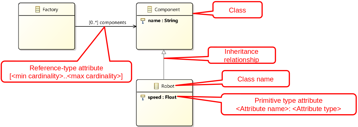
Using the class inheritance concept covered in class, create classes for each type of factory component. Add the attributes you consider useful for these types.

Modelling the factory and its components

Create a class to model the factory and its components. Do not forget reference-type attributes, such as the various components contained within the factory.

Overriding the object display method

Override the toString() method in each class to customize their Console output.

Instantiating and displaying a factory

To test your model:

Create a test class containing a main() method.
In the main() method, instantiate a robotic factory with:
(a) Three rooms, each containing:
- A production area with a production machine.
(b) Three robots.
(c) One charging station.
Display the factory in the Console.
Verify that the string representation of the factory is correct.

TP 5: Visualizing the robotized factory model through interfaces

Overview

In the previous practical session, we modelled the structure of the robotized factory for which we want to develop a simulator. We created an object model of the factory. In this session, we will modify this model to make it visualizable through a graphical interface provided to you. To do so, your model must implement the Java interfaces provided by this graphical interface.

The graphical interface is very simple. The only thing it can do is display two-dimensional (2D) geometric shapes of rectangular, oval, or polygonal forms, in various colours, with different line styles (dashed and thickness) on a drawing canvas.

As seen in class, an interface defines a perspective or a property descriptor for the classes that implement it. Thus, the provided graphical interface provides Java interfaces specifying a simple 2D shape viewpoint. Each component of the robotized factory can indeed be represented as a 2D shape on a canvas. Therefore, the classes in your model need only implement the provided 2D shape interfaces for the graphical interface to display them.

This set of interfaces provided by the graphical interface serves as a contract between the model and the graphical interface for displaying the model. This way of integrating different software components is a common programming practice.

In this lab, you will learn to:

The graphical interface for shape visualization

Download the graphical interface library for shape visualization (canvas viewer), which can be found here. This library, named canvas-viewer.jar, is essentially a set of compiled Java classes (.class files) that can be used by other Java applications.
Open the canvas-viewer.jar file with a file compression utility like 7-Zip. You will see that it is simply an archive containing .class files arranged in the same directory structure as the class packages. You will also find .java files, allowing you to view the source code of the graphical interface and even set breakpoints to understand what happens using a debugger.

Configuring the simulator project to use the graphical interface library

In the project or package browser in Eclipse, select your simulator project, right-click, and click New > Folder to create a directory named libs.
Move the canvas-viewer.jar file to this directory (you can also directly drag and drop the file from your operating system's file browser into the project browser in Eclipse).
Select your simulator project, right-click, and click Properties.
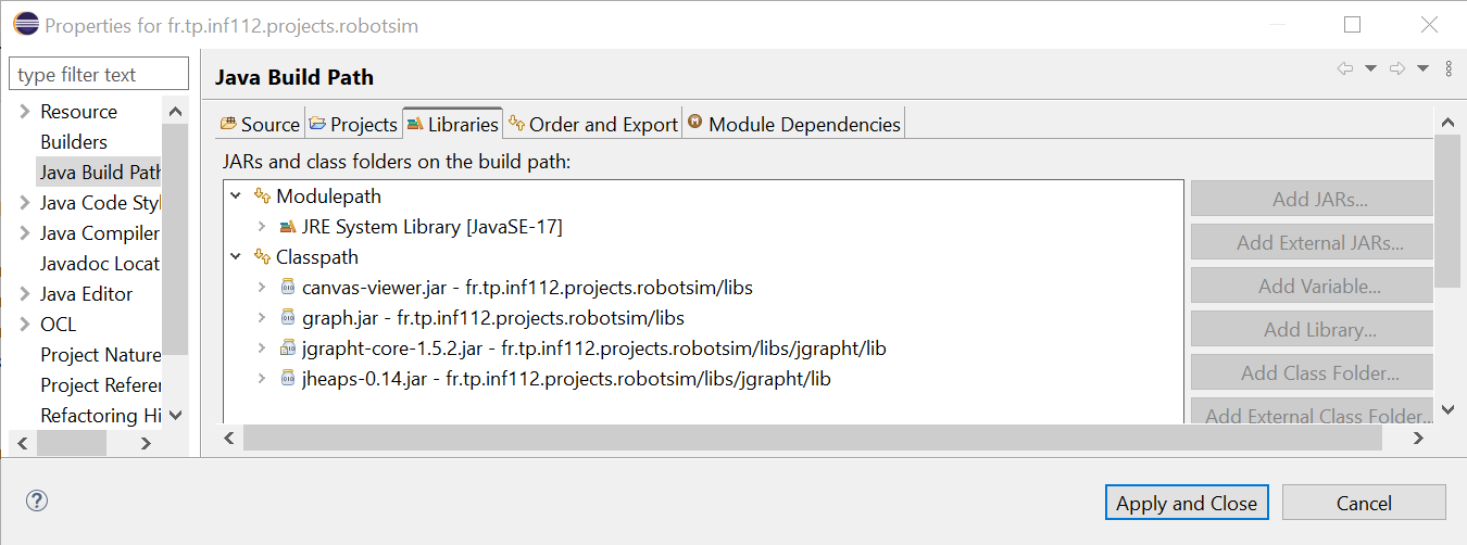
In the dialogue box that appears, select the Java Build Path section, then the Libraries tab on the right side of the window. Select Classpath, then click the Add Jars... button and navigate to the canvas-viewer.jar file you added in the libs directory.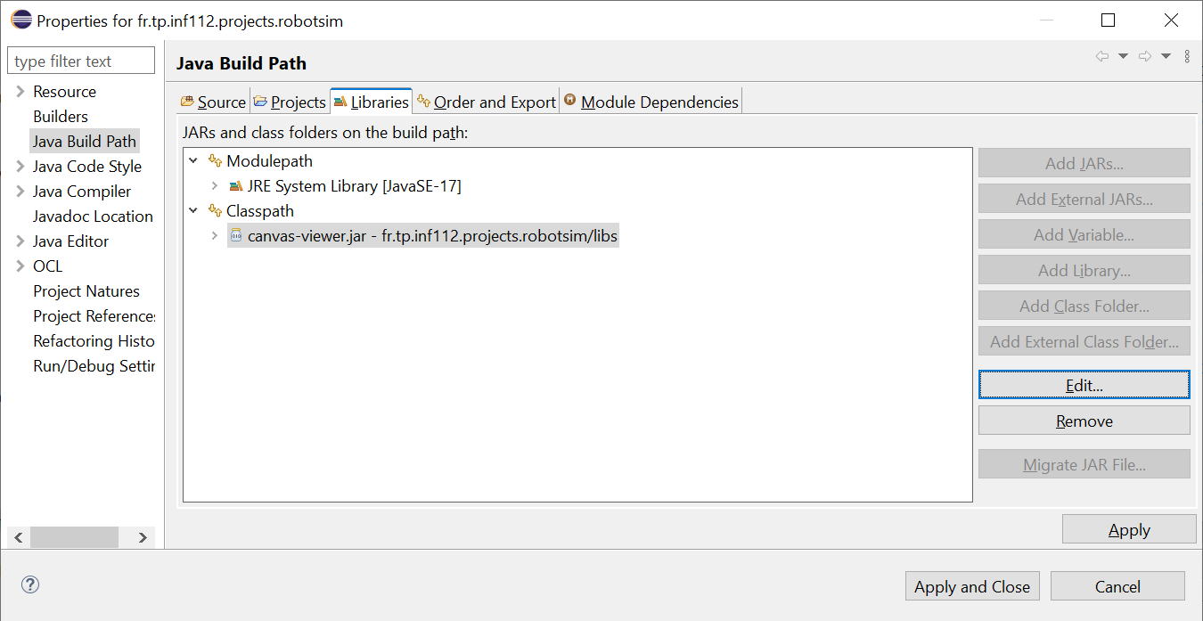
In the package explorer (or project browser), expand the Referenced Libraries branch. You will see the canvas-viewer.jar library you just added to the project.
You will also see the packages provided by this library. Open the packages fr.tp.inf112.projects.canvas.model and fr.tp.inf112.projects.canvas.model.impl.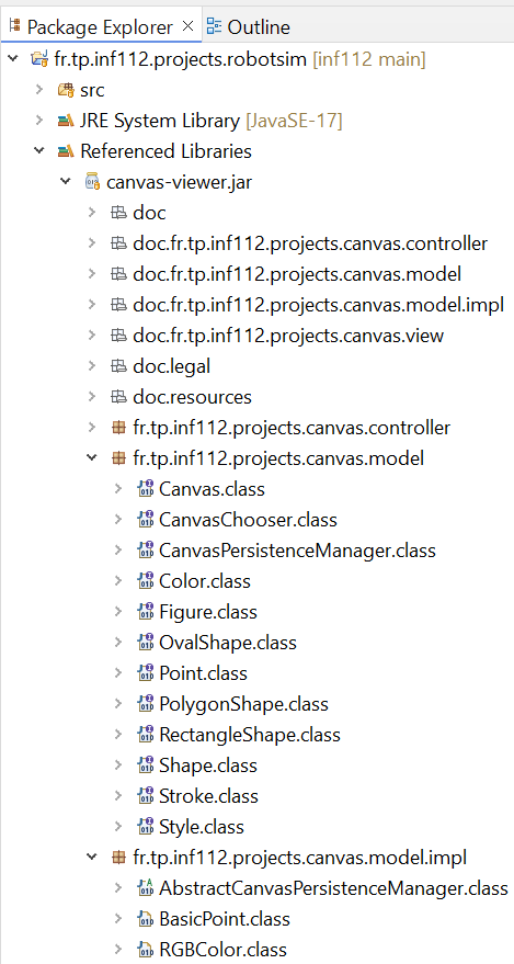
Examine the contents of these packages. In fr.tp.inf112.projects.canvas.model you will find interfaces such as Canvas, Figure, Style, and Shape.
- The Canvas interface describes canvas properties such as its name, width, height, and a collection of shapes to display on the canvas.
- The Figure interface describes 2D shape properties such as its name, position on the canvas ($x$ and $y$ coordinates), style (characterized by colour and contour), and shape, as described by the Shape interface.
- The graphical interface can display only three types of shapes, whose properties are described by the sub-interfaces RectangleShape, OvalShape, and PolygonShape.
To make them easier to use, all these interfaces include Javadoc documentation explaining the various methods required by the interfaces.

Note 1: In fr.tp.inf112.projects.canvas.view you will find the classes that implement the graphical interface used to visualize your robotized factory model. Understanding these classes is unnecessary, as graphical interfaces are not part of this course curriculum.

Implementing the canvas interfaces with the robotized factory model

To display your model in the graphical interface, you must determine which interfaces the classes of your robotized factory model should implement. For example, the factory, which consists of a layout where the components of the factory are positioned, can be seen as a Canvas. Similarly, any component of the robotized factory can be represented by a 2D geometric shape (or figure).

Thus, your abstract Component class must implement the Figure interface:
```
public abstract class Component implements Figure
```

Name and position of the shape on the canvas

The Figure interface requires a name (getName() method) for the shape, displayed on the top-left corner of the shape on the canvas. It also requires the coordinates of the shape to know where to draw it on the canvas.

Style of the shape

The Figure interface also requires knowing the display style of the shape. This style is characterized by a background colour for the shape (getBackgroundColor() method) and the contour characteristics (thickness, dash, colour, as described by the Stroke interface).

Shape of the shape

As mentioned earlier, the graphical interface can only draw shapes of rectangular (RectangleShape), oval (OvalShape), or polygonal (PolygonShape) forms.

For each concrete subclass of the Component class, you must determine the desired shape and define implementation classes for these shapes.
Then, each component must define the getShape() method of the Figure interface to return an instance of the implementation corresponding to the chosen shape for the component.

For example: Since the robots in the factory are circular, your Robot class will return an instance of an implementation class of OvalShape, while the Room or Area classes, corresponding to rectangular components, will return instances of an implementation class of RectangleShape.
Do the same for each class component of your model that needs to be visualized by the graphical interface, except for the class representing the robotized factory, which will be considered rectangular.

The canvas

Indeed, this class should instead implement the Canvas interface, which represents the container for shapes. Note that the Canvas interface specifies a Collection<Figure> getFigures() method. Since all the factory components implement the Figure interface, you can directly return the attribute of your Factory class containing the components.

However, you may need to cast this reference as follows:

public Collection<Figure> getFigures() {
    return (Collection) components;
}

Launching the graphical interface

Examine the CanvasViewer class in the fr.tp.inf112.projects.canvas.view package of the graphical interface library (file canvas-viewer.jar). One of the constructors of this class takes a single parameter: an instance of a class implementing the Canvas interface. This is the constructor you will use to launch the graphical interface.
To this end, create a class named SimulatorApplication to represent the simulator application linking the model and the graphical interface.
In this class, create a main() method.
In this method, instantiate a factory model as in the previous session, which contains:
- 3 rooms, each containing a workspace with a production machine,
- 3 robots, and
- 1 charging station.
Then, instantiate the CanvasViewer class provided by the graphical interface, providing it with the factory you just created.
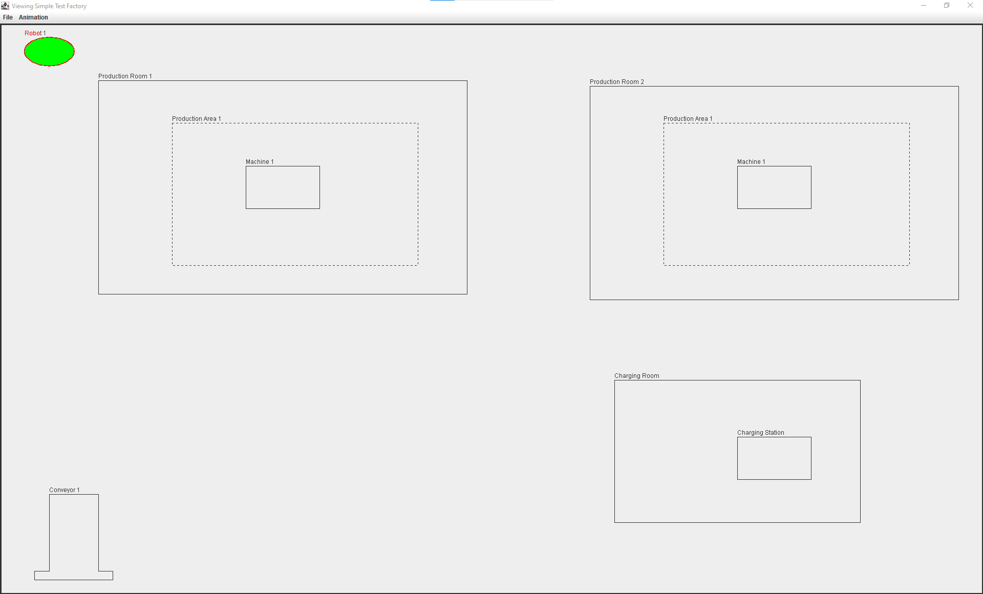
Run the main() method.
Verify that your model is correctly displayed in the graphical interface, as illustrated by the following figure.

Note 2: It should be noted that none of the actions defined by the graphical interface menus will work (they will be disabled) except for the action of quitting the application. These actions will be defined in the next practical session when you implement the controller interface of the model-view-controller design pattern, which we will explain in class first.

TP 6: Simulating the robotic factory model using MVC

Overview

In the previous practical session, you modified your robotic factory object model to implement the model interfaces of the graphical Canvas Viewer interface (canvas-viewer.jar) provided to you. This allowed visualizing your model as 2D figures with different colours, styles, and geometric shapes.

In this lab, you will define the behavioural view of your model to simulate it. Then, to visualize this simulation using the Canvas Viewer interface, you will need to create a class that implements the controller interface, enabling control over the display and simulation of your model.

In this lab, you will learn to:

Specifying the model behaviour

You will now model the behavioural part of the robotic factory. This involves defining methods in the various classes of factory components to describe how their states, represented by the values of their attributes, evolve over time and in response to events in the factory.

First, define a new method named behave() in the Component class of your model. Initially, this method will be empty. Each factory component whose state can change over time will override this method to specify its behaviour when the factory operates.
In the Factory class, override the behave() method inherited from the Component class. For each component in the factory, call the behave() method of its subcomponent. Thus, any method overridden by a subclass of Component will be executed, simulating the specific behaviour of each subclass.

Moving robots

Specify the behaviour of the Robot class. Initially, this behaviour involves moving from one component to another within the factory. To do this, add an attribute to the Robot class to hold a list of components the robot must visit as it moves through the factory.
In the same Robot class, override the behave() method inherited from Component.
- Within this behave() method, retrieve the first component from the list of components to be visited by the robot. Then, call a method named move() that you will define as described in the next section.
- Before calling move(), verify if the robot has reached the target component by checking if its position matches that of the component.
- If so, retrieve the next component in the list and direct the robot towards it. When the end of the list is reached, the robot must return to the first component in the list of components to visit.
In the Robot class, define the move() method.
- In this method, increment (or decrement, as needed) the robot’s x and y coordinates by a value defined by an attribute specifying the robot’s speed, so that the robot moves closer to the component to visit. For now, assume there are no obstacles between the robot and the component it is heading toward.

Observers

Open the canvas-viewer.jar library located in the libs directory of your Eclipse project for the robotic factory simulator. Within the package fr.tp.inf112.projects.canvas.controller, you will find the CanvasViewerController, Observable, and Observer interfaces.
Open the CanvasViewer class from the canvas-viewer.jar library. You will notice that this class, which serves as the view (and thus the observer) in the MVC pattern, implements the Observer interface. This interface defines only one method, modelChanged(), which must be called by your model every time its data changes, so that the view(s) can refresh the data and keep the display consistent with the model's data.
Examine the body of the modelChanged() method in the CanvasViewer class. It simply calls the repaint methods of the menu bar and the panel that displays the shapes from your model. When displaying the menus in the menu bar, the Start Animation and Stop Animation menus will be enabled or disabled depending on whether your model is currently running a simulation, as determined by a call to the isAnimationRunning() method from the controller interface presented later in this document.

Implementing the `Observable` interface

To notify the view when its data changes, the model must implement the Observable interface:

public class Factory extends Component implements Canvas, Observable { ... }

This interface contains methods to add and remove observers. To implement them, declare an attribute in the Factory class to hold its observers.

Notify the view(s) when the model’s data has changed

Since the simulator follows an MVC architecture, you will need to modify your model’s code so that any change in its data (such as the coordinates of a moving robot, for example) can notify the views that have been registered as observers of the model. This way, the views can refresh and display the updated data from the model.

To achieve this, in the Factory class, you will need to create a notifyObservers() method that will call the modelChanged() method of each observer that has been registered with the model.
This notifyObservers() method should be called by the model whenever its data is modified, for all the classes in your model that need to be visualized by the graphical interface.

There are several ways to achieve this. A simple approach is to add an attribute of type Factory to the Component class, so that each component can call the notifyObservers() method of the Factory class whenever its data is changed through its setter methods.

Implementing the `Controller` interface

Open the CanvasViewerController interface from the canvas-viewer.jar library. Create a SimulatorController class implementing this interface. Pass an instance of this class to the CanvasViewer constructor for visualizing your model.
The CanvasViewerController interface inherits from the Observable interface. This means that the view registers with the model indirectly through the controller. Therefore, in your controller, you will need to maintain a reference to the model and implement the methods of the Observable interface by calling the corresponding methods of the model.

By reading the Javadoc of the methods in the CanvasViewerController interface, provide implementations for the required methods. The controller is responsible for starting and stopping the simulation using the startAnimation() and stopAnimation() methods, which are called by the view when the corresponding menus are selected. Additionally, a call to the isAnimationRunning() method allows the view to check whether the simulation is currently running, so it can manage the activation of the animation control menus.

To implement the startAnimation(), stopAnimation(), and isAnimationRunning() methods in your controller class, add an attribute to the Factory class to keep track of whether the simulation has started or not.
Also, add the startSimuation(), stopSimulation(), and isSimulationStarted() methods to the Factory class to manage this attribute. Do not forget to notify the observers when the value of this attribute changes.

In the startAnimation() method of the controller, copy the following code:

factoryModel.startSimulation();

while (factoryModel.isSimulationStarted()) {
    factoryModel.behave();

    try {
        Thread.sleep( 200 );
    }
    catch (InterruptedException ex) {
        ex.printStackTrace();
    }
}

The graphical interface will take care of launching the simulation of your model in a dedicated task (thread or lightweight process) to avoid interrupting its display, which runs in a specific JVM task called the Event Dispatch Thread.

The sleep() method is used to wait for 200 milliseconds between each execution of the behave() method of the factory, to prevent the animation from running too quickly and allowing the user to better visualize the simulation. This value can be changed if needed.

Note the try-catch instructions used to handle the InterruptedException, which will be thrown if another task interrupts the task in which the simulator is running.

Finally, implement the stopAnimation() and isAnimationRunning() methods in your controller class by delegating these operations to the model.

Launching the simulation

To test your simulation, follow these steps:

In a test class, instantiate a factory containing: 1 robot, 2 machines, and 1 charging station.
Add these three components to the list of components to be visited by the robot.
Instantiate the CanvasViewer class from the graphical interface, this time using the constructor that takes a controller as a parameter.
Verify that your robot moves correctly, visiting the two machines and the charging station sequentially.

TP 7: Save the robotic factory model

Overview

In the previous practical session, you modified your object-oriented model of the robotic factory so that the robots could move from one component of the factory to another. You also implemented the MVC interfaces provided by the Canvas Viewer graphical interface so that the movements of these robots could be automatically visualized.

In this practical session, you will develop the data access layer (or persistence layer) for your simulator in order to store the data of the robotic factory model on permanent storage (SSD or database). This data will then be able to be re-read when the simulator is restarted.

This persistence layer will rely on various Java classes used to handle input and output operations, such as reading and writing data to files in either text or binary format.

In this lab, you will learn to:

Introduction to input / output in Java and data persistence

Read the presentation on input and output in Java available here.
Then read the presentation on data persistence here.

Update the `Canvas Viewer` library

First, download the latest version of the Canvas Viewer graphical interface, which can be found here.
Then replace your current version with this new one. You will notice differences in the canvas model interfaces, which will be explained later in this document.

The controller interface

The CanvasViewerController interface has a new method called getPersistenceManager(), as declared in the following code:

/**
* Returns the persistence manager to be used to persist this canvas
* model into a data store.
* @return A non {@code null} {@code CanvasPersistenceManager}
* implementation for the desired data storage kind
* (file, database, etc.).
*/

CanvasPersistenceManager getPersistenceManager();

This method should return an object of a class that implements the CanvasPersistenceManager interface.

Implement the persistence interface

Examine the documentation for the CanvasPersistenceManager interface. As seen in the presentation on data persistence, this interface specifies method signatures for reading, writing (persisting), and deleting a canvas model.

For this simulator, we will implement a data persistence layer that relies on the file system of the computer running the program.

To simplify the implementation of the CanvasPersistenceManager interface, create a class that extends the abstract class AbstractCanvasPersistenceManager. This class is provided by the Canvas Viewer library.

The `CanvasChooser` interface

The AbstractCanvasPersistenceManager class contains an attribute of type CanvasChooser, and its constructor takes an object of this type as a parameter. Examine the CanvasChooser interface and its documentation. It specifies a method chooseCanvas(), which returns a string that uniquely identifies a canvas.

It is not necessary to provide a class that implements the CanvasChooser interface. Since the models will be stored in the computer's file system, you can simply instantiate the FileCanvasChooser class, which implements CanvasChooser, and is provided by the Canvas Viewer library.

The FileCanvasChooser class allows browsing the computer's file system and selecting a file whose expected extension can be specified by a constructor parameter. When a user of the Canvas Viewer graphical interface selects the menu File > Open Canvas, the FileCanvasChooser object will be used to present a list of files and folders to the user, who can then browse them to choose a model to visualize.

Model a unique identifier for the model

To store your models in the file system (which acts as a database here), each instance of your factory model should provide a string that will serve as its unique identifier in the file system. To this end, the getId() and setId() methods have been added to the Canvas interface, so that your class representing the robotic factory (Factory), which implements the Canvas interface, will need to provide an attribute for the identifier as well as accessors for this attribute.

When saving the model via the Canvas Viewer graphical interface, the FileCanvasChooser object will also be used so that the user can choose an existing file name from the file system or enter a new file name. This identifier retrieved from the FileCanvasChooser object will then be assigned to the factory model by calling the setId() method of your class. It will be composed of the file name and its path within the folder hierarchy.

Make the model classes serializable

To simplify the representation of your model in a file, you will use data serialization, as seen in the course presentation on data input and output.

To do this, any class in your model that needs to be saved must implement the Serializable interface. Modify the classes in your model to implement this interface. Note that this interface is a marker interface, meaning it declares no methods and only serves to mark classes.

However, some data in the classes may not need to be preserved / saved between executions of the program. This is the case for the model's observers. It is better not to store these objects, especially since they are instances of Java graphical interface classes, which are not always serializable.

Therefore, use the transient keyword to declare that the observer attribute should not be serialized.
Do not forget to modify the instantiation of the attribute to use lazy instantiation, as no class constructor will be called during the deserialisation of the object, as discussed in the presentation on input-output.
Then, do the same for any other attributes of your model classes that should not be serialized.

Implement persistence methods

The abstract class AbstractCanvasPersistenceManager does not provide the body for the read(), persist(), and delete() methods of the CanvasPersistenceManager interface.

You need to implement these methods in your persistence class using object serialization streams ObjectInputStream and ObjectOutputStream, as introduced in the presentation on input and output operations.
For the delete() method, a simple approach is to instantiate an object of the java.io.File class and call the delete() method on this object.

Test the model persistence

To test the persistence of your model, run the simulator as you did in the previous lab session.
Use the Open Canvas and Save Canvas submenus from the File menu in the Canvas Viewer interface and verify that you can save the model to disk and then correctly reload it in the graphical interface.

Set up application logging

As we saw in class, it is preferable to use a logging library to display the program’s execution traces instead of directly using the system console output. This allows storing the traces in other media, such as files.

In this part of the exercise, you will set up logging both to the console and in a log file using and configuring the JDK’s logger.

Configure the logger

As seen in class, logging can be configured in Java code or via a configuration file. For any JRE installation, a default configuration file is provided in the installation directory of the JRE. You will copy this file into a directory in your simulator project, then modify it to adjust the logger configuration to your needs.

As shown in the following screenshot, open the directory of your simulator project to locate the installation directory of the JRE System Library in your computer's file system. From this directory, navigate to a subdirectory named conf and copy the logging.properties file.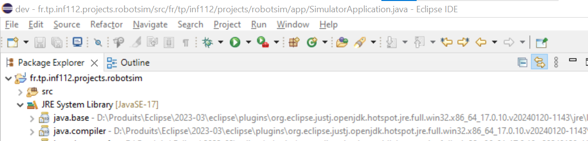
Create a directory named config in your project and place the previously retrieved logging.properties file in it, as shown in the following screenshot.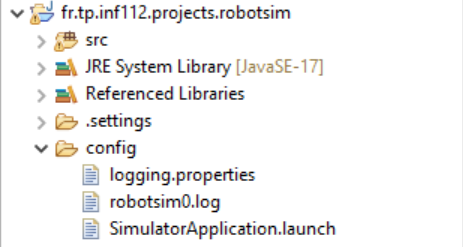
Open the logging.properties file in Eclipse and modify it so that two handlers are used: a first handler that writes to the console and a second one that writes to a file, as illustrated in the following screenshot.
Next, as shown in the screenshot below, specify the path of the log file so that it is created in the config directory of the simulator project, then save the logger configuration file.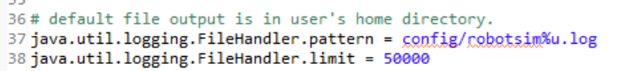
Then, specify the location of the logging configuration file to be used by your simulator. This can be done by setting the value of the java.util.logging.config.file property, as shown in the following screenshot.
Finally, also save your simulator launch configuration in your project. This will make it easier for teachers to evaluate your project, as they can directly use your launch configuration to run your simulator and check its proper functioning. This is done by selecting the Common tab and specifying the directory in the text field of the Shared file option, as shown in the following screenshot.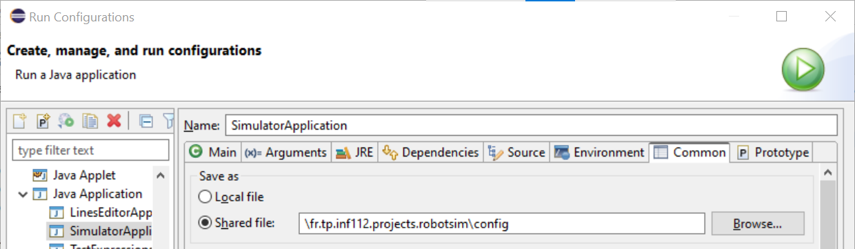

Define a logger object to display messages

In your simulator application's class (SimulatorApplication), create a variable for the logger like the one in the following line.
```
private static final Logger LOGGER = Logger.getLogger(Main.class.getName());
```
Then, display two information messages notifying the start of your simulator, with two different levels of detail: info and config, as shown in the following code.
```
LOGGER.info("Starting the robot simulator...");
LOGGER.config("With parameters " + Arrays.toString(args) + ".");
```

Verify the logger's proper functioning

Run your simulator and observe the messages that appear in the console.
In the Eclipse project explorer, refresh the config folder. The log file generated by the logger should appear.
Open it and verify the messages written in it. Are all the messages properly displayed in both the console and the log file? If not, why?
Examine the contents of the logging.properties file and change the logging level to config. Verify that both messages are correctly displayed in the log file.
Then, set a finer logging level (such as fine) and restart the simulator. Do the logging messages still appear? You will notice that several messages from the graphical interface now appear at this level of detail. If the simulator's messages no longer appear, check the value of the java.util.logging.FileHandler.limit property and refer to its documentation to fix the problem.

Note 1: Note that the log file is written in XML format, while the data is written in a different format in the console. How do you explain this difference?

TP 8: Avoiding obstacles

Overview

During Lab 6, you implemented the Model-View-Controller (MVC) architecture to visualize any changes in the model data through the graphical interface. You also defined a very simple behavior for the factory robots, consisting of visiting a list of components within the factory. These movements did not take into account the various obstacles in the factory, such as room walls, for instance.

In this lab, you will refine the robots' movements to navigate around obstacles in the factory. To achieve this, you will use a trajectory calculation library that will be provided to you.

In this lab, you will learn to:

Trajectory calculation

There are several methods for trajectory calculation in robotics, as well as in video games. The approach you will implement for this project is inspired by what is described here.

The first step involves creating a map of the space in which the robots operate. This map will determine the occupancy of the various objects within the represented space. A typical approach is to discretize this space, as illustrated by the following figure.

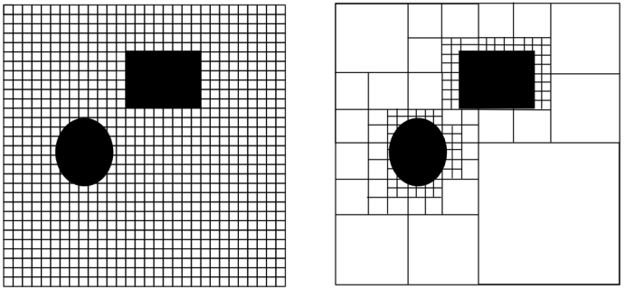
The left part of the figure represents a discretization of the space into squares, whose size will depend on the precision required for the simulation, as well as the memory and processing resources allocated to this simulation. Indeed, very fine discretization will allow for highly precise trajectory determination but will require more memory and computation time. That said, in case of problems, it is possible to optimize the memory required to store the map by representing it as a k-d tree, such that only areas containing obstacle boundaries are mapped, as illustrated by the right side of the previous figure.

Once the space has been discretized, it can be viewed as a graph. Thus, each square can be seen as a node of the graph, and for each square, an edge will be added between the node of that square and the node of each of its adjacent squares. However, not all adjacent squares will necessarily be considered. If an adjacent square coincides with an obstacle, no edge will be added between the node of the square and the obstacle square, making the obstacle nodes inaccessible.

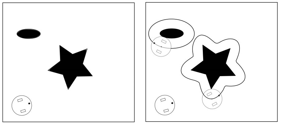
It will therefore be necessary to detect obstacles to determine whether an adjacent square should be connected by an edge or not. Here again, several approaches can be used to detect obstacles. A frequently used approach involves considering the moving object as a point and increasing the size of the objects to be avoided by half the maximum dimension of the moving object, as illustrated by the following figure.

However, this requires calculations that can become quite complex, depending on the shape of the objects. There are various libraries, such as Apache Commons Geometry, that allow modelling geometric shapes, but their use remains complicated.

A very common approach in video games is to approximate any shape with a similar-sized shape whose contours are simpler, such as a circle or a rectangle. This latter approximation is the one you will use in this lab. An explanation of this method can be found here.

Once the space is viewed as a graph, well-known algorithms such as Dijkstra’s algorithm can be used to find the shortest path in the graph. This pathfinding process, illustrated by an animation here, is what you will use in this lab.

Just as with the graphical visualization interface, you will use an existing library to integrate into your project for calculating the shortest path.

There are several other trajectory calculation algorithms, such as A*, which adds heuristics to Dijkstra’s algorithm to avoid performing a complete search on all graph nodes. More recently, algorithms employing machine learning have been developed to calculate robot trajectories.

Creating a trajectory calculation interface

As previously discussed, trajectory calculation is a relatively complex topic, and there are several algorithms with different properties. Thus, it is preferable to encapsulate the trajectory calculation in a dedicated class, as recommended by the single responsibility principle in object-oriented design. Moreover, since there are multiple algorithms, your factory model should only be aware of a trajectory calculation interface, thereby decoupling your factory model from technical dependencies related to specific algorithms. This will make it easier to change the algorithm without modifying the model classes.

To achieve this, create an interface named FactoryPathFinder. In this interface, define a method signature named findPath(). This method will take two parameters: the first being a source component and the second a target component, both serving as the starting and ending nodes of the shortest path to be calculated.

The findPath() method will return a list of objects of type Position, a simple class encapsulating the x and y coordinates in a plane. If the Position class does not yet exist in your model, you can create it and modify your model so that it stores component coordinates as instances of this Position class.

Next, modify your Robot class to allow it to be provided with an object of type FactoryPathFinder. Update the behaviour of your Robot class (specifically the behave() method) to use the FactoryPathFinder object. Each time the component to be visited changes, calculate a new trajectory for this new target, and at each simulation cycle, move the robot to the next position in the previously calculated trajectory until the target is reached. Then update the new target, and so on.

Implementing the trajectory calculation interface

Now, develop a class implementing the FactoryPathFinder interface. This class will implement Dijkstra’s algorithm by calling an existing graph modeling library.

Two graph modelling libraries

Choose the library you will use from the two libraries described in the following subsections.

The `JGraphT` library

JGraphT is a very rich and widely used library for various graph processing tasks. It is also very well-documented and open-source. It provides several classes to model different types of graphs, including directed ones, for example. If you choose this library, you will use the DefaultDirectedGraph class. This class is generic (like the List interface and its classes such as ArrayList), and can therefore be used with any classes of your choice to model the vertices and edges. You will need to use your own class to represent the vertices and use the DefaultEdge class, provided by JGraphT, to represent the edges. You will use the DijkstraShortestPath class and its findPathBetween() method to calculate the shortest path between two vertices.

Simulator project setup in Eclipse (JGraphT)

The JGraphT library can be downloaded here (under the DOWNLOAD menu). Add this library to your project in Eclipse as described in TP 5 for the canvas-viewer.jar library. Configure your project to use both jgrapht-core-<version>.jar and jheaps-<version>.jar files from JGraphT as illustrated by the following screenshot.

The JGraphT documentation can be found here, with a Hello JGraphT section to help you get started if you choose to use this library.

The "homemade" graph library

This library, simpler but more limited than JGraphT, provides various interfaces modelling a graph (Graph), its vertices (Vertex), and its edges (Edge), along with basic implementations of these interfaces. For this exercise, you will use the GridGraph, GridVertex, and GridEdge classes, which implement the previous interfaces and facilitate the conversion of a grid, such as the layout of a robotic factory, into a graph.

This library also contains a class named DijkstraAlgorithm, which provides a static method called findShortestPath(). This method takes as parameters an object of type Graph and two objects of type Vertex, representing the start and end vertices of the path. It returns a list of adjacent vertices, starting with the start vertex and ending with the end vertex, defining the shortest path between these vertices.

Simulator project setup in Eclipse ("homemade" library)

The "homemade" Graph library can be downloaded here. Add this library to your project in Eclipse as described earlier for JGraphT. Configure your project to use the graph.jar file as illustrated by the previous screenshot.

Approach to using the graph library

To use the Canvas Viewer graphical interface to visualize your model, you have had the Canvas and Figure programming interfaces implemented by your model. These interfaces define a viewpoint on your model. In the case of the Dijkstra algorithm, you will use a different approach, that of model transformation. This approach is defined as the automatic generation of one or more target models from one or more source models, and is essential in model-driven engineering in order to use different model analysis tools, whose input formats are not the same as that of the source model.

The reason for this choice, compared to the viewpoint approach used to visualize your robotic factory model, is that for this simulator, we wish to evaluate different types of trajectory computation algorithms, which can be easily achieved by using different implementation classes of the FactoryPathFinder interface. This minimizes the coupling between the classes of the robotic factory model and the pathfinding classes.

This is not the case for visualizing the robotic factory, which uses only one type of visualization. By directly implementing the Canvas interfaces in the robotic factory model, it becomes strongly coupled with the Canvas Viewer library. In contrast, using the viewpoint approach provides better performance than model transformation because there is no need to reconvert all the factory objects into canvas objects each time the data changes, which would make the visualization much less fluid.

Transforming a robotic factory model into a graph

To calculate the shortest path between a robot and its target, you will need to develop Java code to transform a robotic factory model into a graph model. You will first need to instantiate an object of the class representing a graph from the graph library you have chosen (see previous sections). Then, you will need to instantiate graph vertex and edge objects to represent the cells of the factory layout.

The class representing the vertices must be able to store the position of the corresponding cell in the factory layout in order to convert the calculated path into a list of positions for the robots to visit, as defined by the findPath() method of the FactoryPathFinder interface.

If you use JGraphT, you can use any class of your choice to represent the vertices and use the DefaultEdge class from JGraphT to represent the edges. If you use the "homemade" graph library, the vertex class must be GridVertex or a subclass of it, and the vertex and edge classes will be GridVertex and GridEdge, respectively.

Creating the graph for the robotic factory

For each cell of the factory, you will need to create a vertex by instantiating the chosen vertex class, which will store the position of the associated cell. Once all the graph vertices have been created, you will need to build the edges between these vertices. As an approximation, consider that the robots can only move in the x (width) and y (height) directions. Thus, for a given cell, only the four adjacent cells to the left, right, above, and below will be connected to the central cell by an edge. For now, assume there are no obstacles in the factory.

Calculating the shortest path

In the findPath() method of your class implementing the FactoryPathFinder interface, call the shortest path search method using the appropriate classes from the chosen library. Then, you will need to convert the list of vertices returned into a list of positions in the factory, which the findPath() method must return as required by the FactoryPathFinder interface.

Testing the functionality of trajectory calculation, without obstacles

The development of this part of the simulator being more complex than previous assignments, use an incremental development approach. First, test your trajectory calculation algorithm without considering the obstacles in the factory.

To do this, instantiate a factory containing a robot and two machines, each located in a space within its own room. Each room will be equipped with a door. Add a charging station in its own room. Add both machines and the charging station to the list of components to be visited by the robot. Launch the graphical interface and verify that your robot moves correctly, visiting both machines and the charging station in succession, without considering the obstacles.

Detecting obstacles

To circumvent obstacles, you should not add an edge if the adjacent cell is located on an object that should not be crossed by the robot, as illustrated by this animation.

A good way to proceed is to delegate the decision of whether a cell contains a blocking object to the factory object, as it knows all the components. For example, you can add an overlays() method to your Component class, which will take an object of the class representing the graph vertices as a parameter and determine if these two objects overlap. To this end, you can approximate the shape of the factory components using a simple shape of a size similar to the actual shape, as described in this tutorial on game development.

The factory, when asked if a vertex overlaps one of its components, will iterate through all the components to call the overlays() method and determine if any component is an obstacle. If so, no edge will be constructed to this vertex.

The overlays() method can be redefined in subclasses of components to account for their specificities. Consider that a room consists of walls, of a certain thickness, and doors as subcomponents. A wall constitutes an obstacle and cannot be overlapped. A door only constitutes an obstacle if it is closed.

Consider that areas do not have walls and can therefore be traversed. Also, assume for simplicity that machines, conveyors, and charging stations can be traversed by robots.

Don’t forget to handle the case where no path exists between a robot and its target. Consult the documentation of the graph library to understand what will be returned by the algorithm in this case. You can indicate this state of the robot being blocked visually in the graphical interface by changing the style of the figure returned by the robot or its label, for example.

Also, handle the exception case where another robot is located in the next cell a robot needs to move to. In this case, the robot should not move, and will only continue its trajectory on the next call to the behave() method if the cell has been freed.

Testing the functionality of obstacle detection

Relaunch the simulator with the model described earlier and verify that your robot correctly avoids obstacles by entering rooms through their doors if they are open. Also, test with multiple robots and ensure that they do not collide with each other.

Further steps

The following two exercises are optional and will not be evaluated.

Allow robots to move diagonally

Modify your code so that robots can move diagonally, in addition to along the x and y axes. What do you notice? Do robots still take the shortest path? Propose a solution to this problem.

Managing robot energy

Define an energy level for the robots. For a robot, decrease this energy level by a fixed amount with each move. When the energy level is low, the robot will calculate a trajectory to each charging station and decide to continue its work if the remaining energy is sufficient. Otherwise, it will head toward the nearest charging station. The behaviour of the charging station, upon detecting that a robot is present, will be to recharge the robot until the battery is full, at which point the robot can continue its work.

Eclipse IDE: Eclipse IDE Java Developers download
Oracle JDK: Oracle JDK downloads
OpenJDK installs: OpenJDK install instructions

Course downloads

Canvas Viewer (canvas-viewer.jar): Download canvas-viewer.jar
Graph helper library (graph.jar): Download graph.jar
Additional material: I/O: INF112 I/O (PDF)
Additional material: Persistence: INF112 Persistence (PDF)

Libraries & references

JGraphT: JGraphT official site
Apache Commons Geometry: Apache Commons Geometry
Path planning (MIT notes): MIT path planning notes
Dijkstra (explanation/animation): Dijkstra algorithm (Wikipedia, French)
k-d tree (explanation): k-d tree (Wikipedia, French)
Aditional tutorial of Git: Introduction to Git

Utilities & optional tools

7-Zip: 7-Zip download
Copilot for Eclipse (optional): Copilot4Eclipse marketplace

Inspiration for the course project

Hasso-Plattner Institute: CPSLab resources (HPI)

Object-Oriented Java - Labs