TP 8: Avoiding obstacles

Overview

During Lab 6, you implemented the Model-View-Controller (MVC) architecture to visualize any changes in the model data through the graphical interface. You also defined a very simple behavior for the factory robots, consisting of visiting a list of components within the factory. These movements did not take into account the various obstacles in the factory, such as room walls, for instance.

In this lab, you will refine the robots' movements to navigate around obstacles in the factory. To achieve this, you will use a trajectory calculation library that will be provided to you.

In this lab, you will learn to:

• Model the workspace as a graph and compute shortest paths
• Provide a pluggable FactoryPathFinder and integrate a graph library
• Detect obstacles and adapt paths to avoid them

Trajectory calculation

There are several methods for trajectory calculation in robotics, as well as in video games. The approach you will implement for this project is inspired by what is described here.

The first step involves creating a map of the space in which the robots operate. This map will determine the occupancy of the various objects within the represented space. A typical approach is to discretize this space, as illustrated by the following figure.

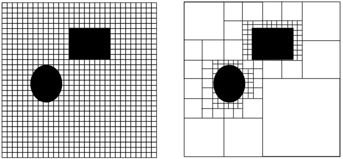
The left part of the figure represents a discretization of the space into squares, whose size will depend on the precision required for the simulation, as well as the memory and processing resources allocated to this simulation. Indeed, very fine discretization will allow for highly precise trajectory determination but will require more memory and computation time. That said, in case of problems, it is possible to optimize the memory required to store the map by representing it as a k-d tree, such that only areas containing obstacle boundaries are mapped, as illustrated by the right side of the previous figure.

Once the space has been discretized, it can be viewed as a graph. Thus, each square can be seen as a node of the graph, and for each square, an edge will be added between the node of that square and the node of each of its adjacent squares. However, not all adjacent squares will necessarily be considered. If an adjacent square coincides with an obstacle, no edge will be added between the node of the square and the obstacle square, making the obstacle nodes inaccessible.

It will therefore be necessary to detect obstacles to determine whether an adjacent square should be connected by an edge or not. Here again, several approaches can be used to detect obstacles. A frequently used approach involves considering the moving object as a point and increasing the size of the objects to be avoided by half the maximum dimension of the moving object, as illustrated by the following figure.

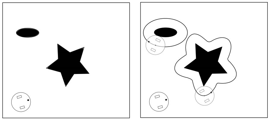
However, this requires calculations that can become quite complex, depending on the shape of the objects. There are various libraries, such as Apache Commons Geometry, that allow modelling geometric shapes, but their use remains complicated.

A very common approach in video games is to approximate any shape with a similar-sized shape whose contours are simpler, such as a circle or a rectangle. This latter approximation is the one you will use in this lab. An explanation of this method can be found here.

Once the space is viewed as a graph, well-known algorithms such as Dijkstra’s algorithm can be used to find the shortest path in the graph. This pathfinding process, illustrated by an animation here, is what you will use in this lab.

Just as with the graphical visualization interface, you will use an existing library to integrate into your project for calculating the shortest path.

There are several other trajectory calculation algorithms, such as A*, which adds heuristics to Dijkstra’s algorithm to avoid performing a complete search on all graph nodes. More recently, algorithms employing machine learning have been developed to calculate robot trajectories.

Creating a trajectory calculation interface

As previously discussed, trajectory calculation is a relatively complex topic, and there are several algorithms with different properties. Thus, it is preferable to encapsulate the trajectory calculation in a dedicated class, as recommended by the single responsibility principle in object-oriented design. Moreover, since there are multiple algorithms, your factory model should only be aware of a trajectory calculation interface, thereby decoupling your factory model from technical dependencies related to specific algorithms. This will make it easier to change the algorithm without modifying the model classes.

To achieve this, create an interface named FactoryPathFinder. In this interface, define a method signature named findPath(). This method will take two parameters: the first being a source component and the second a target component, both serving as the starting and ending nodes of the shortest path to be calculated.

The findPath() method will return a list of objects of type Position, a simple class encapsulating the x and y coordinates in a plane. If the Position class does not yet exist in your model, you can create it and modify your model so that it stores component coordinates as instances of this Position class.

Next, modify your Robot class to allow it to be provided with an object of type FactoryPathFinder. Update the behaviour of your Robot class (specifically the behave() method) to use the FactoryPathFinder object. Each time the component to be visited changes, calculate a new trajectory for this new target, and at each simulation cycle, move the robot to the next position in the previously calculated trajectory until the target is reached. Then update the new target, and so on.

Implementing the trajectory calculation interface

Now, develop a class implementing the FactoryPathFinder interface. This class will implement Dijkstra’s algorithm by calling an existing graph modeling library.

Two graph modelling libraries

Choose the library you will use from the two libraries described in the following subsections.

The JGraphT library

JGraphT is a very rich and widely used library for various graph processing tasks. It is also very well-documented and open-source. It provides several classes to model different types of graphs, including directed ones, for example. If you choose this library, you will use the DefaultDirectedGraph class. This class is generic (like the List interface and its classes such as ArrayList), and can therefore be used with any classes of your choice to model the vertices and edges. You will need to use your own class to represent the vertices and use the DefaultEdge class, provided by JGraphT, to represent the edges. You will use the DijkstraShortestPath class and its findPathBetween() method to calculate the shortest path between two vertices.

Simulator project setup in Eclipse (JGraphT)

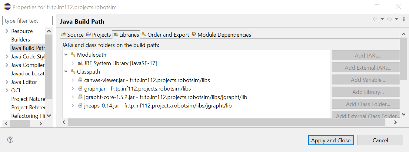
The JGraphT library can be downloaded here (under the DOWNLOAD menu). Add this library to your project in Eclipse as described in TP 5 for the canvas-viewer.jar library. Configure your project to use both jgrapht-core-<version>.jar and jheaps-<version>.jar files from JGraphT as illustrated by the following screenshot.

The JGraphT documentation can be found here, with a Hello JGraphT section to help you get started if you choose to use this library.

The "homemade" graph library

This library, simpler but more limited than JGraphT, provides various interfaces modelling a graph (Graph), its vertices (Vertex), and its edges (Edge), along with basic implementations of these interfaces. For this exercise, you will use the GridGraph, GridVertex, and GridEdge classes, which implement the previous interfaces and facilitate the conversion of a grid, such as the layout of a robotic factory, into a graph.

This library also contains a class named DijkstraAlgorithm, which provides a static method called findShortestPath(). This method takes as parameters an object of type Graph and two objects of type Vertex, representing the start and end vertices of the path. It returns a list of adjacent vertices, starting with the start vertex and ending with the end vertex, defining the shortest path between these vertices.

Simulator project setup in Eclipse ("homemade" library)

The "homemade" Graph library can be downloaded here. Add this library to your project in Eclipse as described earlier for JGraphT. Configure your project to use the graph.jar file as illustrated by the previous screenshot.

Approach to using the graph library

To use the Canvas Viewer graphical interface to visualize your model, you have had the Canvas and Figure programming interfaces implemented by your model. These interfaces define a viewpoint on your model. In the case of the Dijkstra algorithm, you will use a different approach, that of model transformation. This approach is defined as the automatic generation of one or more target models from one or more source models, and is essential in model-driven engineering in order to use different model analysis tools, whose input formats are not the same as that of the source model.

The reason for this choice, compared to the viewpoint approach used to visualize your robotic factory model, is that for this simulator, we wish to evaluate different types of trajectory computation algorithms, which can be easily achieved by using different implementation classes of the FactoryPathFinder interface. This minimizes the coupling between the classes of the robotic factory model and the pathfinding classes.

This is not the case for visualizing the robotic factory, which uses only one type of visualization. By directly implementing the Canvas interfaces in the robotic factory model, it becomes strongly coupled with the Canvas Viewer library. In contrast, using the viewpoint approach provides better performance than model transformation because there is no need to reconvert all the factory objects into canvas objects each time the data changes, which would make the visualization much less fluid.

Transforming a robotic factory model into a graph

To calculate the shortest path between a robot and its target, you will need to develop Java code to transform a robotic factory model into a graph model. You will first need to instantiate an object of the class representing a graph from the graph library you have chosen (see previous sections). Then, you will need to instantiate graph vertex and edge objects to represent the cells of the factory layout.

The class representing the vertices must be able to store the position of the corresponding cell in the factory layout in order to convert the calculated path into a list of positions for the robots to visit, as defined by the findPath() method of the FactoryPathFinder interface.

If you use JGraphT, you can use any class of your choice to represent the vertices and use the DefaultEdge class from JGraphT to represent the edges. If you use the "homemade" graph library, the vertex class must be GridVertex or a subclass of it, and the vertex and edge classes will be GridVertex and GridEdge, respectively.

Creating the graph for the robotic factory

For each cell of the factory, you will need to create a vertex by instantiating the chosen vertex class, which will store the position of the associated cell. Once all the graph vertices have been created, you will need to build the edges between these vertices. As an approximation, consider that the robots can only move in the x (width) and y (height) directions. Thus, for a given cell, only the four adjacent cells to the left, right, above, and below will be connected to the central cell by an edge. For now, assume there are no obstacles in the factory.

Calculating the shortest path

In the findPath() method of your class implementing the FactoryPathFinder interface, call the shortest path search method using the appropriate classes from the chosen library. Then, you will need to convert the list of vertices returned into a list of positions in the factory, which the findPath() method must return as required by the FactoryPathFinder interface.

Testing the functionality of trajectory calculation, without obstacles

The development of this part of the simulator being more complex than previous assignments, use an incremental development approach. First, test your trajectory calculation algorithm without considering the obstacles in the factory.

To do this, instantiate a factory containing a robot and two machines, each located in a space within its own room. Each room will be equipped with a door. Add a charging station in its own room. Add both machines and the charging station to the list of components to be visited by the robot. Launch the graphical interface and verify that your robot moves correctly, visiting both machines and the charging station in succession, without considering the obstacles.

Detecting obstacles

To circumvent obstacles, you should not add an edge if the adjacent cell is located on an object that should not be crossed by the robot, as illustrated by this animation.

A good way to proceed is to delegate the decision of whether a cell contains a blocking object to the factory object, as it knows all the components. For example, you can add an overlays() method to your Component class, which will take an object of the class representing the graph vertices as a parameter and determine if these two objects overlap. To this end, you can approximate the shape of the factory components using a simple shape of a size similar to the actual shape, as described in this tutorial on game development.

The factory, when asked if a vertex overlaps one of its components, will iterate through all the components to call the overlays() method and determine if any component is an obstacle. If so, no edge will be constructed to this vertex.

The overlays() method can be redefined in subclasses of components to account for their specificities. Consider that a room consists of walls, of a certain thickness, and doors as subcomponents. A wall constitutes an obstacle and cannot be overlapped. A door only constitutes an obstacle if it is closed.

Consider that areas do not have walls and can therefore be traversed. Also, assume for simplicity that machines, conveyors, and charging stations can be traversed by robots.

Don’t forget to handle the case where no path exists between a robot and its target. Consult the documentation of the graph library to understand what will be returned by the algorithm in this case. You can indicate this state of the robot being blocked visually in the graphical interface by changing the style of the figure returned by the robot or its label, for example.

Also, handle the exception case where another robot is located in the next cell a robot needs to move to. In this case, the robot should not move, and will only continue its trajectory on the next call to the behave() method if the cell has been freed.

Testing the functionality of obstacle detection

Relaunch the simulator with the model described earlier and verify that your robot correctly avoids obstacles by entering rooms through their doors if they are open. Also, test with multiple robots and ensure that they do not collide with each other.

Further steps

The following two exercises are optional and will not be evaluated.

Allow robots to move diagonally

Modify your code so that robots can move diagonally, in addition to along the x and y axes. What do you notice? Do robots still take the shortest path? Propose a solution to this problem.

Managing robot energy

Define an energy level for the robots. For a robot, decrease this energy level by a fixed amount with each move. When the energy level is low, the robot will calculate a trajectory to each charging station and decide to continue its work if the remaining energy is sufficient. Otherwise, it will head toward the nearest charging station. The behaviour of the charging station, upon detecting that a robot is present, will be to recharge the robot until the battery is full, at which point the robot can continue its work.

Develop an automated door

Implement behaviour for the doors so that they automatically open when a robot arrives and close after the robot passes.